Your browser does not fully support modern features. Please upgrade for a smoother experience.
Please note this is an old version of this entry, which may differ significantly from the current revision.
Heart rate variability (HRV) has emerged as an essential non-invasive tool for understanding cardiac autonomic function over the last few decades. This can be attributed to the direct connection between the heart’s rhythm and the activity of the sympathetic and parasympathetic nervous systems. Different researchers have employed various dimensionality reduction methods to decrease the feature dimension of the HRV features.
- cannabis
- heart rate variability
- signal analysis
- feature selection
1. Principal Component Analysis (PCA)
PCA is a renowned unsupervised ML technique that employs an orthogonal conversion algorithm to alter many associated features to a set of unrelated features identified as principal components [58]. The orthogonal alteration is performed utilizing the eigenvalue breakdown of the covariance matrix, which is produced using the features of the specified signal. PCA selects the dimensions containing the most significant information while discarding the dimensions containing the least important information. This, sequentially, assists to lessen the dimensionality of the data [70]. The samples in the PCA-based approach are placed in a lower-dimensional space, such as 2D or 3D. Because it makes use of the signal’s variation and changes it to alternate dimensions with lesser characteristics, it is a useful tool for attribute choosing. However, the transformation preserves the variance of the signal components.
The PCA technique is generally executed via either the matrix or data methods. The matrix method uses all the data contained in the signal to compute the variance–covariance structure and represents it in the matrix form. Here, the raw data are transformed using matrix operations through linear algebra and statistical methodologies. And yet, the data process works directly on the information and matrix-based operations are not required [70]. Various features like the mean, deviation, and covariance are involved in implementing a PCA-based algorithm. The mean or average (µ) value of the data samples (xi) calculated during the implementation of PCA is given in Equation (16) [70].
 where xi represents the data samples.
The deviation (𝜙𝑖) for the dataset can be mathematically expressed using Equation (17) [70].
 where xi represents the data samples, and µ represents the deviation.
Covariance (C) determines the variable value that has changed randomly and how much it has deviated from the original data [71]. This value may be either positive or negative and is based on the deviation it has gone through in the previous steps. The covariance matrix is calculated using the deviation formula and then transposing it [70].
 where A= [Φ1, Φ2... Φn] is the set of deviations observed from the original data.
In order to apply PCA for dimensionality reduction purposes, the eigenvalues and the respective eigenvectors of the covariance matrix C need to be computed [70]. Among all the eigenvectors (say m), the first k number of eigenvectors with the highest eigenvalues are selected. This corresponds to the inherent dimensionality of the subspace regulating the signal. The rest of the dimensions (m-k) contain noise. For the representation of the signal using principal components, the signal is projected into the k-dimensional subspace using the rule given in Equation (19) [70].
 where U represents an m × k matrix whose columns comprise the k eigenvectors.
PCA helps to obtain a set of uncorrelated linear combinations as given in the matrix form below (Equation (20)) [71].
 where Y = (Y1, Y2, …, Yp)T, Y1 represents the first principal component, Y2 represents the second principal component, and so on. A is an orthogonal matrix having ATA = I.
2. Kernel PCA (K-PCA)
K-PCA is an extension of the principal component analysis (PCA) approach that may be used with non-linear information by employing several filters, including linear, polynomial, and Gaussian [58]. This method transforms the input signal into a novel feature space employing a non-linear transformation. A kernel matrix K is formed through the dot product of the newly generated features in the transformed space, which act as the covariance matrix [72]. For the construction of the kernel matrix, a non-linear transformation (say φ(x)) from the original D-dimensional feature space to an M-dimensional feature space (where M >> D) is performed. It is then assumed that the new features detected in the transformed domain have a zero mean (Equation (21)) [73]. The covariance matrix (C) of the newly projected features has an M × M dimension and is calculated using Equation (22) [73]. The eigenvectors and eigenvalues of the covariance matrix represented in Equation (23) are calculated using Equation (24) [73]. The eigenvector term vk in Equation (23) is expanded using Equation (24) [73]. By replacing the term vk in Equation (23) with Equation (24), we obtain the expression in Equation (25) [73]. By defining a kernel function, 𝑘(𝑥𝑖,𝑥𝑗)=𝜙(𝑥𝑖)𝑇𝜙(𝑥𝑗), and multiplying both sides of Equation (25), we obtain Equation (26) [73]. Using matrix notation for the terms mentioned in Equation (26) and solving the equation, we obtain the principal components of the kernel (Equation (27)) [73]. If the projected dataset does not have a zero mean feature, the kernel matrix is replaced using a Gram matrix represented in Equation (28) [73].


 where k = 1, 2, …, M, vk = kth eigenvector, and λk corresponds to its eigenvalue.


 where aki represents the coefficient of the kth eigenvector and k(xl, xi) represents the kernel function.
 where 1N represents the matrix with N × N elements that equals 1/N.
Lastly, PCA is executed on the kernel matrix (K). In the K-PCA technique, the principal components are correlated, meaning the eigenvector is projected in an orthogonal direction with more variance than any other vectors in the sample data. The mean-square approximation error and the entropy representation are minimal in the principal components. Identifying new directions using the kernel matrix enhances accuracy compared to the traditional PCA algorithm.
3. Independent Component Analysis (ICA)
An Independent Component Analysis (ICA) is an analysis system used in ML to separate independent sources from the input mixed signal, which is also known as blind source separation (BSS) or the blind signal parting problem [74,75]. The test signal is transformed linearly into components that are independent of each other. In ICA, the hidden factors are analyzed, viz., sets of random variables. ICA is more similar to PCA. ICA is proficient in discovering the causal influences or foundations. Before the implementation of the ICA technique on the data, a few preprocessing steps, like whitening, centering, and filtering, are usually performed on the data to improve the value of the signal and eliminate the noise.
3.1. Centering
Centering is regarded as the most basic and essential preprocessing step for implementing ICA [74]. In this step, the mean value is subtracted from each data point to transform the data into a zero-mean variable and simplify the implementation of the ICA algorithm. Later, the mean can be estimated and added to the independent components.
3.2. Whitening
A data value is referred to as white when its constituents become uncorrelated, and their alterations are equal to one. The purpose of whitening or sphering is to transform the data so that their covariance matrix becomes an identity matrix [74]. The eigenvalue decomposition (EVD) of the covariance matrix is a popular method for the implementation of whitening. Whitening eliminates redundancy, and the features to be estimated are also reduced. Therefore, the memory space requirement is reduced accordingly.
3.3. Filtering
The filtering-based preprocessing step is generally used depending on the application. For example, if the input is time-series data, then some band-pass filtering may be used. Even if we linearly filter the input signal xi(t) and obtain a modified signal xi*(t), the ICA model remains the same [74].
3.4. Fast ICA Algorithm
Fast ICA is an algorithm designed by AapoHyvärinen at the Helsinki University of Technology to implement ICA effectively [62]. The Fast ICA algorithm is simple and requires minimal memory space. This algorithm assumes that the data (say x) are already subjected to preprocessing like centering and whitening. The algorithm aims to find a direction (in terms of a unit vector w) so that the non-Gaussianity of the projection wTx is maximized, where wTx represents an independent component. The non-Gaussianity is computed in negentropy, as discussed in [74]. A fixed-point repetition system is used to discover the highest non-Gaussianity of the wTx projection. Since several independent components (like w1Tx, …, wnTx) need to be calculated for the input data, the decorrelation between them is crucial. The decorrelation is generally achieved using a deflation scheme developed using Gram–Schmidt decorrelation [74]. The estimation of independent components is performed one after another. This is similar to a statistical technique called a projection pursuit, which involves finding the possible number of projections in multi-dimensional data. The Fast ICA algorithm possesses the advantage of being parallel and distributed, and possesses computational ease and less of a memory requirement.
4. Singular Value Decomposition (SVD)
Another approach that builds on PCA is singular value decomposition (SVD), which uses attribute elimination to cut down on overlap [58]. Its consequence is a smaller number of components than PCA but it retains the maximum variance of the signal features. The process is based on the factorization principle of real or complex matrices of linear algebra. This method performs the algebraic transformation of data and is regarded as a reliable method of orthogonal matrix decomposition. The SVD method can be employed to any matrix, making it more stable and robust. This method can be used for a dimension reduction in big data, thereby reducing the time for computing [76]. SVD is used for a dataset having linear relationships between the transformed vectors.
The SVD algorithm is a powerful method for splitting a system into a set of linearly independent components where each component has its energy contribution. To understand the principle of SVD, let us consider a matrix A of dimensions M × N and another matrix U of M × M dimensions. The vectors of A and U are assumed to be orthogonal. Further, let us assume another matrix S, which has a dimension of M × N. Another orthogonal matrix, VT, having a dimension of N × N is also assumed. Then, matrix A is represented by Equation (29) using the SVD method [77].
 where the columns of U are called left singular vectors, and those of V are called right singular vectors.
5. Self-Organizing Map (SOM)
The self-organizing map (SOM) or the Kohonen map corresponds to a neural network that helps in dimensionality-reduction-based feature selection. The map here signifies the low-dimensional depiction of the features of the specified signal. SOM is based on unsupervised ML with node arrangement as a two-dimensional grid. Each node in the SOM is connected with a weighted vector to make computing easier [78]. SOM implements the notion of a race network, which aims to determine the utmost alike detachment between the input vector and the neuron with weight vector wi. The architecture of SOM comprising both the input vector ‘x’ and output vector ‘y’ is shown in Figure 7.
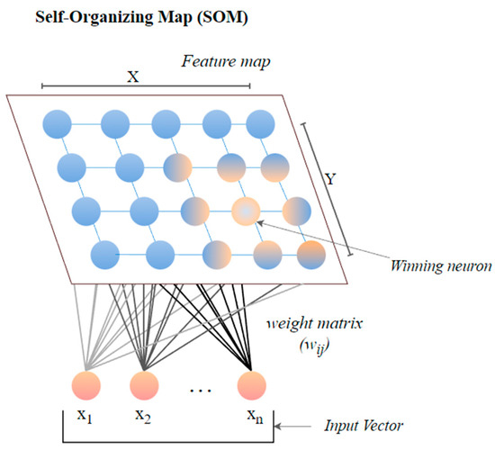
Figure 7. The architecture of SOM.
The size of the weight vector ‘wi’ in SOM is controlled using the learning rate functions like the linear, the inverse of time, and the power series as given in Equations (30)–(32) [79].


 where T represents the number of iterations and t is the order number of a certain it.
It is distinct from the other ANNs in the case of implementing the neighborhood function. A neighborhood function is a function that computes the rate of neighborhood change around the winner neuron in a neural network. Usually, the bubble and Gaussian functions (Equations (33) and (34)) are used as neighborhood functions in SOM.

 where Nc = the index set of neighbor nodes close to the node with indices c, Rc, and Rij = indices of wc and wij, respectively, and ηcij = the neighborhood rank between nodes wc and wij.
This entry is adapted from the peer-reviewed paper 10.3390/a16090433
This entry is offline, you can click here to edit this entry!