Dynamic Groundwater Contamination Vulnerability Assessment Techniques: History
Please note this is an old version of this entry, which may differ significantly from the current revision.
Contributor: , , , ,

Assuring the quantity and quality of groundwater resources is essential for the well-being of human and ecological health, society, and the economy. For the last few decades, groundwater vulnerability modeling techniques have become essential for groundwater protection and management. Groundwater contamination is highly dynamic due to its dependency on recharge, which is a function of time-dependent parameters such as precipitation and evapotranspiration. Therefore, it is necessary to consider the time-series analysis in the “approximation” process to model the dynamic vulnerability of groundwater contamination. 

  • groundwater contamination
  • spatiotemporal vulnerability assessment
  • time-dependent variables
  • modeling techniques

1. Introduction

Water naturally contains several different dissolved inorganic constituents such as calcium, magnesium, sodium, potassium, chloride, sulfate, carbonate, etc. In addition, minor constituents may be present in the water, such as iron, manganese, fluoride, nitrate, and strontium. It may also contain trace elements, such as arsenic, lead, cadmium, and chromium, in amounts of only a few micrograms per liter. The presence of these constituents or elements is dependent on the Earth’s strata holding the water. They are important from a water-quality perspective [1]. But when the natural occurrence elevates the concentration (acceptable for a specific purpose) of these elements, they harm human health and are called pollutants. As these contaminants originate from rock material by leaching or withering [2], this is called geogenic contamination. Geogenic contamination can be defined as a phenomenon caused by geologic process-es. Conversely, groundwater contamination is mainly a combination and sequence of surface and subsurface processes. These processes are directly involved in groundwater recharge. As the climate controls precipitation and evapotranspiration, climate change’s impact alters the progression of recharge by directly speeding up or delaying the surface and subsurface processes.
Contamination and pollution are not the same. The first is the presence of a sub-stance in an amount above the background concentration level. On the other hand, pollution is contamination that results in or can create adverse biological effects to the resident community. Deeper aquifers may be less affected by biological and chemical substances; however, contamination of shallow groundwater sources has become endemic due to human interference with the near-surface or subsurface water flow pathways. Agricultural fertilizers, pesticides, solvents, and chemicals are used in the manufacturing industries, mining, energy production, commercial applications, and pharmaceuticals industry, and human waste-induced pathogens lead to chronic contamination of shallow and deep ground-water worldwide [3]. On a regional scale, groundwater can also be contaminated by geogenic factors (naturally occurring elevated concentrations of certain elements) through adsorption/desorption kinetics associated with soil or rock minerals such as arsenic and fluoride [3]. In addition, groundwater quality is also susceptible to various climate change effects, such as changing precipitation patterns, increasing evapotranspiration (ET), etc.
Pesticides’ fates and transport in the subsurface under agricultural land use are sensitive to climate change-induced changes in rainfall seasonality and intensity, as well as changed rates of recharge [4][5]. Furthermore, climate change and increasing global urbanization may also increase the risk of flooding. This urban flooding increases the loading of common urban pollutants like oil, solvents, and sewage into groundwater [6][7]. In short, the groundwater system is continuously changing due to its dynamic interactions with physical and socio-economic systems. The observed or expected groundwater state changes often diverge from what is most desirable, and it is far beyond the scope of a single individual to control these changes. Groundwater is a common pool resource but can cause significant discrepancies between the interests and preferences of individuals compared to those of a local community. These reasons motivate and justify increased studies and interventions in groundwater resource management [8].
“Vulnerability is not an absolute characteristic, but rather a relative, non-measurable, dimensionless property indicating where contamination is most likely to occur” [9]. The concept of aquifer vulnerability was introduced by [10]. It was defined as “the possibility of percolation and diffusion of contaminants from the surface into natural water table reservoirs, under natural conditions”. Ref. [11] described groundwater vulnerability as “an intrinsic property of a groundwater system that depends on the sensitivity of that system to human and/or natural impacts”. According to [12], the vulnerability of groundwater can be intrinsic or specific depending upon the nature of the contamination. Intrinsic vulnerability is a function of hydrogeological factors by which pollutants can reach and diffuse into groundwater when introduced to the surface [11]. Intrinsic vulnerability is sensitive to natural or geogenic contamination and does not consider anthropogenic activities [13]. Specific vulnerability refers to the susceptibility to a particular and/or a group of pollutants based on contaminant properties, attenuation processes, and transport characteristics [14][15]. Specific vulnerability refers to the impact of specific land use. In other words, this integrates the risk of the contaminants generated by human activities [9].

Spatiotemporal Assessment of Groundwater Vulnerability

Traditionally, models of groundwater contamination were based on the “static” hypothesis that groundwater’s vulnerability to contamination is not time-dependent. However, groundwater’s vulnerability is inherently dependent on groundwater recharge, which is mainly controlled by precipitation and evapotranspiration as well as the surface- and subsurface-level structure of the ground. Therefore, groundwater recharge is highly time-dependent, and strategies for evaluating future groundwater vulnerability in a changing climate and land-use scenarios must consider the “dynamic” concept of vulnerability [13]. Most environmental processes depend on space and time, with time series and spatial data series being strongly reliant on each other. According to the deterministic theory of spatiotemporal hydrogeological variability, a time series is a systematic pattern that helps to identify the trend/periodic factor/shift and/or the combination thereof [16][17] first introduced the concept of spatiotemporal vulnerability in hydrology. It was defined as “the ability of this system to cope with external, natural and anthropogenic impacts that affect its state and character in time and space”. The application of spatiotemporal analysis became a part of groundwater vulnerability assessment during the last three decades, along with the significant development of quantitative applications in the hydrological domain. Studies have shown that spatiotemporal assessment has evolved as a powerful tool for investigating hydrologic/hydrogeologic time series data for surface and subsurface flows. The time dependency of groundwater’s vulnerability to contamination is already well defined, and many researchers have conducted several studies to analyze groundwater’s temporal vulnerability using various qualitative and quantitative approaches.

2. Dynamic Groundwater Contamination Vulnerability Assessment Techniques

2.1. Porous Aquifer Vulnerability Assessment

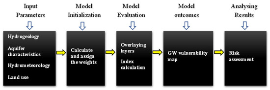
2.1.1. Overlay and Index-Based Models

Overlay and index-based models are mainly subjective/knowledge-based methods. These are the oldest groundwater contamination modeling techniques. The execution of these methods is easy and demands minimal parameters to assess groundwater vulnerability (Figure 1). The index-based models employed in the last decade for the assessment of dynamic groundwater vulnerability assessment are IEA-UEF [18], WQI [19], m-HPI [20], GOD [21], Pesticide DRASTIC [22], DRASTIC [23], GWV [24][25], and NPI [26].
Figure 1. Flowchart for the overlay and index models used to assess groundwater contamination.
Two revolutionary indices (DRASTIC and GOD) are still popular among researchers who employ index-based analysis in their spatiotemporal vulnerability studies. However, these have been modified and/or integrated according to the needs of the studies. Ref. [22] integrated statistical analysis, such as hierarchical cluster analyses (HCA), and discriminant analysis to establish the relationships between the locations and to determine the seasonal effect, respectively. Ref. [23] integrated the analytical hierarchy process (AHP) theory with DRASTIC to modify the weightings and ratings based on the experience and knowledge of specialists or users. AHP was also incorporated by [21] using the GOD modeling technique. As GOD is a static model, the assessment of the spatiotemporal variations was computed using ANOVA. During the last decade, besides vulnerability, many spatiotemporal groundwater quality assessments have studied water quality index (WQI), the immune evolutionary algorithm–universal exponential formula (IEA-UEF), modified heavy metal pollution index (m-HPI), and nitrate pollution index (NPI). The WQI [19] and an updated and integrated version of the WQI called the IEA-UEF [18] assessed the groundwater quality samples collected for a certain period to investigate the contaminants influencing the groundwater quality and/or to specify the groundwater quality zones. Two new approaches, m-HPI [20] and NPI [26], were introduced in order to analyze the spatiotemporal trend of heavy metal and nitrate, respectively, based on the collected groundwater samples for a given period. These models (WQI, IEA-UEF, m-HPI, and NPI) employed kriging and/or inverse distance weighting (IDW) method to fulfill the need for spatial trend analysis. All of these models are suitable for groundwater quality assessment. Understanding the groundwater quality status and tracking the pollution trend is crucial. However, these trends are meaningless when not incorporated with the physico-hydrological parameters. It is essential to know the geogenic or anthropogenic history of the aquifer systems and the geophysical processes to draw meaningful conclusions regarding the analysis and policy making. Therefore, these models are lacking in terms of defining the dynamic groundwater vulnerability. Refs. [24][25] presented a long-term predictive model. They predicted the groundwater vulnerability for three periods: past (1961–1990), present (2011–2040), and future (2041–2070). They employed the groundwater vulnerability (GWV) method to assess and predict the long-term vulnerability. This method uses various important climatic parameters to evaluate and predict the groundwater vulnerability scenario while considering climate change. 

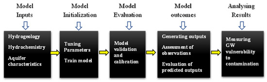
1.1.2. Statistical Models

Statistical models are based on data-driven methods, ranging from conditional probability analysis and regression to descriptive statistics. Statistical involvement allows objective methods to determine the relationship between the level of contamination and predictor factors. Over the last decade, many attempts have been initiated to calculate groundwater’s vulnerability to contamination using statistical modeling techniques (Figure 2).
Figure 2. General flowchart for the statistical model to assess groundwater contamination.

Spatial Interpolations

In groundwater vulnerability assessment, spatial interpolation uses information on sample location points to predict and map the unsampled locations. Depending on their probabilistic nature, spatial interpolation techniques can be divided into deterministic (e.g., IDW) and geostatistical (e.g., Kriging) approaches. Ref. [27] employed disjunctive kriging (DK), along with ordinary kriging and cokriging, to assess the probability of non-point source groundwater contamination under the influence of agricultural land use. They collected groundwater samples according to the summer crop cycle from 2004 to 2006. The results indicate that interannual climate variation and fertilization control nitrate contamination. Therefore, from an agri-environmental perspective, this method can achieve a reliable outcome for the decision-makers. Ref. [28] employed ordinary point kriging to assess the spatiotemporal groundwater contamination in the Mediterranean region. They monitored the groundwater table depth and contours, pH, EC, and NO3 during the pre-monsoon (June) and post-monsoon (October) seasons in 2009 and 2010 from 220 monitoring wells. The outcome reported how rainfall patterns can change the evapotranspiration pattern, which controls the amount of NO3 leaching (higher temperature and lower relative humidity can increase evapotranspiration and minimize the risk of NO3 leaching).

Multivariate Statistics

In the past decade, many multivariate analyses were conducted to analyze the spatiotemporal distribution of contaminants in the groundwater. Principal component analysis (PCA) is one of the most significant and widely used parameter-identifying tools and data reduction techniques for almost all environmental studies. It found that in the recent past, PCA integrated with factor analysis (FA), hierarchical cluster analysis (HCA), regressions, or spatial interpolation methods was intensively used in the vulnerability assessment of groundwater contamination. Ref. [29] presented a GIS-based study by combining PCA and IDW to investigate the nitrogen sources in groundwater under various land use scenarios. Ref. [30] combined PCA and FA to track the urban pollution source and the concentration level. FA was employed to reduce the involvement of less significant parameters within each component. This reduction procedure involved extracting a different set of varifactors by rotating the axes defined by the PCA extraction. A K-means-based cluster analysis (CA) was employed on the FA-extracted varifactors to analyze the similarities in the water quality. Ref. [31] employed PCA to track the source and transport of chlorate in the groundwater under agricultural land use. Ref. [32] investigated the spatiotemporal vulnerability of GW quality using a robust PCA (ROBPCA) method. To avoid the drawbacks of classical PCA (such as anomalous observations, overestimating the variance, etc.), they compared and proposed ROBPCA for the measurement of the seasonal and hydro-chemical characteristics of the aquifer. ROBPCA is a useful method for identifying spatiotemporal variations in GW quality when hydro-chemical processes are diverse and anomalous samples are available.

Regression Models

Ref. [33] investigated nitrate contamination using the generalized additive mixed models (GAMMs) suggested by [34]. These regression models are used primarily for spatiotemporal trend identification in complex monitoring data. Ref. [35] employed a combined multiple regression and multi-tracer method to predict the spatiotemporal distribution of nitrate in the groundwater and the factors contributing to its sources. Time series (1980, 1995, and 2000) land use maps were used to estimate the land use pattern at the time of recharge of “young water”. This temporal analysis was conducted using the linear interpolation method [36]. A simple material balance model [37] was fitted to estimate the nitrate concentration mixed by different recharge sources given the known amount of water recharged into shallow aquifers.

Artificial Intelligence

Ref. [38] proposed a feed-forward multilayer artificial neural network (ANN) to investigate the pollution sources in terms of duration of activity, magnitude, and location. A back propagation neural network (BPNN) was employed to identify the source characteristics. The Latin hypercube sampling (LHS) approach generated temporal varying source fluxes. These outputs were used in groundwater flow and the transport simulation model. The information generated through this process was used in the ANN model-building processes. Breakthrough curves (BTC) were also obtained for the specific contamination scenarios. The parameters of the BTC were used as inputs for the ANN model.

Spatial Autocorrelation

Ref. [39] evaluated the spatiotemporal trend of fluoride concentration by combining two different statistical methods: Moran’s I [40] and Local Indicators of Spatial Association (LISA) [41]. LISA is a distance-based method that quantifies the extent of clustering of the high or low values of the parameter of interest and how the values in the neighboring locations vary within a specified bandwidth (distance). LISA provides a better indication of the clustering of the spatial units by calculating local Moran’s I for each unit.

Bayesian Networks

Ref. [42] introduced an integrated approach to assess the time-dependent vulnerability of groundwater to non-point source contamination. A data-driven Bayesian method (weights of evidence (WofE)) was employed to determine the relationship between temporal changes in land use and GW pollution and to forecast future trends. Ref. [43] introduced a new regret-based optimization model to identify the pollution source in the GW system. Groundwater flow and contaminant transport were calculated using MODFLOW and MT3D. A Monte Carlo analysis was employed to measure the impacts of risk and uncertainty in the model parameters and inputs. A Bayesian network model was trained and validated based on the outputs of the Monte Carlo analysis.

Other Statistical Methods

Ref. [44] proposed a detailed decision tree with which to measure the lag time and transport of contaminants in the groundwater. This approach can map the GW vulnerability and comply with the management strategies suggested by the WFD and GWD. Ref. [45] employed the PRACTICAL simulation model [46] to investigate the relationship between nitrate occurrence and contextual variables, i.e., rainfall and recharge. PRACTICAL quantifies the monthly recharge amount by considering a set of contextual parameters in the calculations. Sequential Gaussian simulation was employed to generate simulated scenarios regarding nitrate concentration for each hydrological year to evaluate the values above and below the threshold of 50 mg-NO3/1, and to determine the average of the simulated nitrate concentrations.

Physical/Process-Based Methods

The dynamic concept of GW vulnerability is mainly controlled by various surface and subsurface processes, such as spatial and temporal variation of GW recharge and its storage across multiple flow systems with different residence times. Therefore, these processes should be considered in a GW vulnerability assessment in order to better manage GW resources. Furthermore, processes-based methods can deal with the contaminant’s fate and transport, making them suitable for understanding how anthropogenic activities and climate change may affect this vital source [13].

2.2. Karst Aquifer Vulnerability Assessment

Karst aquifers are one of the most important sources of fresh water, supplying water to fulfil the demand of 25% of the global population [47]. These aquifers provide a significant amount of drinking water in Europe; for some regions, they are the only source of fresh water. The contamination vulnerability of these vital freshwater sources significantly threatens the vast population fulfilling their demand for drinking water. Karst aquifers are susceptible to hydrological changes in the recharge regions. Karst aquifers represent a unique hydrogeological process through the conduit (pipe-like flow system) and diffuse (through fractures and pores) flow systems [13]. Due to these dual characteristics of karst systems, they present more pronounced surface and subsurface interrelationships, making them vulnerable to contaminants in two different ways. Fast travel time and low storage capacity in conduit flow make karsts sensitive to “short-lived” pollutants. On the other hand, in diffuse systems, “persistent” contaminants can be stored and released over a long period of time [13]. Because of these unique vulnerability scenarios, karst aquifers need special attention regarding groundwater vulnerability assessment.

2.2.1. Overlay and Index-Based Method

Ref. [48] evaluated intrinsic and specific vulnerability using the DRASTIC and DRASTIC Pesticide methods. A susceptibility index (SI) was also employed to visualize the temporal changes in specific vulnerability. Due to the typical sub-surface flow system in the karst aquifers, vertical seepage and lateral flow should be considered in order to map the karst groundwater vulnerability in terms of source and resource protection. Ref. [49] measured the spatiotemporal groundwater contamination using the COP method. They integrated the geographically weighted regression (GWR) and used elevation, land-use, geology, and normalized differentiate vegetative index (NDVI) parameters to describe the spatial dynamics of relationships among the variables.

2.2.2. Statistical Method

Ref. [50] developed a GIS tool integrated with the residence time distribution (RTD) model to measure the lumped parameters based on vulnerability mapping parameters. This method links the temporal groundwater quality with the vulnerability concept based on equivalent lumped parameters. This semi-objective method is based on the probability distribution of residence times and can represent a better groundwater vulnerability assessment for decision making.

2.2.3. Process-Based Method

Ref. [13] drew the attention of the hydrogeologist to the variation in spatiotemporal groundwater recharge. They suggested that the consideration of movement tracking of groundwater flow and its discharge at various springs should become essential. It is, therefore, crucial to understand these processes in order to track the water storage and residence time in multiple systems. They suggested a numerical modeling technique for the broader understanding of dynamic karst aquifer vulnerability and its relationship with climate change to achieve better quantification. They employed the recharge, conduit flow, and diffuse flow (RCD) rainfall-discharge model, “RCD-seasonal” [51], to simulate the discharge and substance concentration of the investigated spring. This is a lumped parameter model based on a conceptual model of the karst aquifer system where water flows through three main compartments: the recharge (soil and epikarst system), conduit/fast flow, and diffuse/slow flow systems.

This entry is adapted from the peer-reviewed paper 10.3390/hydrology10090182

References

  1. Fetter, C.W. Applied Hydrogeology, 4th ed.; Prentice Hall: Hoboken, NJ, USA, 2001.
  2. Ghosh, N.C. Geogenic Contamination and Technologies for Safe Drinking Water Supply BT—Water and Sanitation in the New Millennium; Nath, K.J., Sharma, V.P., Eds.; Springer: New Delhi, India, 2017; pp. 81–95.
  3. Lall, U.; Josset, L.; Russo, T. A snapshot of the world’s groundwater challenges. Annu. Rev. Environ. Resour. 2020, 45, 171–194.
  4. Bloomfield, J.P.; Williams, R.J.; Gooddy, D.C.; Cape, J.N.; Guha, P. Impacts of climate change on the fate and behaviour of pesticides in surface and groundwater—A UK perspective. Sci. Total Environ. 2006, 369, 163–177.
  5. Kovalevskii, V.S. Effect of climate changes on groundwater. Water Resour. 2007, 34, 140–152.
  6. Aureli, A.; Taniguchi, M. Groundwater Resources Assesment under the Pressures of Humanity and Climate Changes. Paris. 2006. Available online: https://iwlearn.net/resolveuid/01d776e51f524e6fa99c85b17686aece (accessed on 29 July 2023).
  7. Green, T.R. Linking Climate Change and Groundwater. In Integrated Groundwater Management: Concepts, Approaches and Challenges; Jakeman, A.J., Barreteau, O., Hunt, R.J., Rinaudo, J.D., Ross, A., Eds.; Springer: Berlin/Heidelberg, Germany, 2016; pp. 97–141.
  8. Margat, J.; van der Gun, J. Groundwater around the World: A Geographic Synopsis; CRC Press: Boca Raton, FL, USA, 2013.
  9. Stigter, T.Y.; Ribeiro, L.; Dill, A.M.M.C. Evaluation of an intrinsic and a specific vulnerability assessment method in comparison with groundwater salinisation and nitrate contamination levels in two agricultural regions in the south of Portugal. Hydrogeol. J. 2006, 14, 79–99.
  10. Margat, J. Vulnerabilite des Nappes d’eau Souterraine a la Pollution (Groundwater Vulnerability to Contamination); Bureau de Recherches Géologiques et Minières (BRGM): Orleans, France, 1968.
  11. Vrba, J.; Zaporozec, A. Guidebook on Mapping Groundwater Vulnerability; H. Heise: Hannover, Germany, 1994.
  12. National Research Council. Ground Water Vulnerability Assessment: Predicting Relative Contamination Potential Under Conditions of Uncertainty; The National Academies Press: Washington, DC, USA, 1993.
  13. Butscher, C.; Huggenberger, P. Modeling the temporal variability of karst groundwater vulnerability, with implications for climate change. Environ. Sci. Technol. 2009, 43, 1665–1669.
  14. Doerfliger, N.; Jeannin, P.-Y.; Zwahlen, F. Water Vulnerability Assessment in Karst Environments: A New Method of Defining Protection Areas Using a Multi-Attribute Approach and GIS Tools (EPIK Method); Springer: Berlin/Heidelberg, Germany, 1999.
  15. Gogu, R.C.; Dassargues, A. Current Trends and Future Challenges in Groundwater Vulnerability Assessment Using Overlay and Index Methods; Springer: Berlin/Heidelberg, Germany, 2000.
  16. Haan, C.T. Statistical Methods in Hydrology; Iowa State University Press: Ames, IA, USA, 1977.
  17. Sotornikova, R.; Vrba, J. The concept of vulnerability maps. In Proceedings of the International Conference on Vulnerability of Soil and Groundwater to Pollutants, The Hague, The Netherlands, 30 March–3 April 1987; pp. 471–476.
  18. Nan, Z.; Bo, L.; Changlai, X. Spatio-Temporal variation of groundwater contamination using IEA-UEF in urban areas of Jilin City, North-eastern China. Water Sci. Technol. Water Supply 2016, 16, 1277–1286.
  19. Mahmood, K.; Ul-Haq, Z.; Batool, S.A.; Rana, A.D.; Tariq, S. Application of temporal GIS to track areas of significant concern regarding groundwater contamination. Environ. Earth Sci 2016, 75, 33.
  20. Chaturvedi, A.; Bhattacharjee, S.; Singh, A.K.; Kumar, V. A new approach for indexing groundwater heavy metal pollution. Ecol. Indic. 2018, 87, 323–331.
  21. Misi, A.; Gumindoga, W.; Hoko, Z. An assessment of groundwater potential and vulnerability in the Upper Manyame Sub-Catchment of Zimbabwe. Phys. Chem. Earth 2018, 105, 72–83.
  22. Duttagupta, S.; Mukherjee, A.; Das, K.; Dutta, A.; Bhattacharya, A.; Bhattacharya, J. Groundwater vulnerability to pesticide pollution assessment in the alluvial aquifer of Western Bengal basin, India using overlay and index method. Geochemistry 2020, 80, 125601.
  23. Vu, T.D.; Ni, C.F.; Li, W.C.; Truong, M.H. Modified index-overlay method to assess spatial-temporal variations of groundwater vulnerability and groundwater contamination risk in areas with variable activities of agriculture developments. Water 2019, 11, 2492.
  24. Nistor, M.M. Vulnerability of groundwater resources under climate change in the Pannonian basin. Geo-Spat. Inf. Sci. 2019, 22, 345–358.
  25. Haidu, I.; Nistor, M.M. Groundwater vulnerability assessment in the Grand Est region, France. Quat. Int. 2020, 547, 86–100.
  26. Bahrami, M.; Zarei, A.R.; Rostami, F. Temporal and spatial assessment of groundwater contamination with nitrate by nitrate pollution index (NPI) and GIS (case study: Fasarud Plain, southern Iran). Env. Geochem Health 2020, 42, 3119–3130.
  27. Mendes, M.P.; Ribeiro, L. Nitrate probability mapping in the northern aquifer alluvial system of the river Tagus (Portugal) using Disjunctive Kriging. Sci. Total Environ. 2010, 408, 1021–1034.
  28. Kurunc, A.; Ersahin, S.; Sonmez, N.K.; Kaman, H.; Uz, I.; Uz, B.Y.; Aslan, G.E. Seasonal changes of spatial variation of some groundwater quality variables in a large irrigated coastal Mediterranean region of Turkey. Sci. Total Environ. 2016, 554–555, 53–63.
  29. Li, Q.; Zhang, H.; Guo, S.; Fu, K.; Liao, L.; Xu, Y.; Cheng, S. Groundwater pollution source apportionment using principal component analysis in a multiple land-use area in southwestern China. Environ. Sci. Pollut. Res. 2020, 27, 9000–9011.
  30. Azzellino, A.; Colombo, L.; Lombi, S.; Marchesi, V.; Piana, A.; Andrea, M.; Alberti, L. Groundwater diffuse pollution in functional urban areas: The need to define anthropogenic diffuse pollution background levels. Sci. Total Environ. 2019, 656, 1207–1222.
  31. Mastrocicco, M.; Di Giuseppe, D.; Vincenzi, F.; Colombani, N.; Castaldelli, G. Chlorate origin and fate in shallow groundwater below agricultural landscapes. Environ. Pollut. 2017, 231, 1453–1462.
  32. Jung, H.W.; Yun, S.T.; Kim, K.H.; Oh, S.S.; Kang, K.G. Role of an impermeable layer in controlling groundwater chemistry in a basaltic aquifer beneath an agricultural field, Jeju Island, South Korea. Appl. Geochem. 2014, 45, 82–93.
  33. Mellor, F.P.; Cey, E.E. Using generalized additive mixed models to assess spatial, temporal, and hydrologic controls on bacteria and nitrate in a vulnerable agricultural aquifer. J. Contam. Hydrol. 2015, 182, 104–116.
  34. Wood, S.N. Generalized Additive Models: An Introduction with R; CRC Press: Boca Raton, FL, USA, 2017.
  35. Wang, S.; Tang, C.; Song, X.; Yuan, R.; Han, Z.; Pan, Y. Factors contributing to nitrate contamination in a groundwater recharge area of the North China Plain. Hydrol. Process. 2016, 30, 2271–2285.
  36. Cao, Y.; Tang, C.; Song, X.; Liu, C.; Zhang, Y. Residence time as a key for comprehensive assessment of the relationship between changing land use and nitrates in regional groundwater systems. Environ. Sci. Process. Impacts 2013, 15, 876–885.
  37. Wang, S.; Tang, C.; Song, X.; Wang, Q.; Zhang, Y.; Yuan, R. The impacts of a linear wastewater reservoir on groundwater recharge and geochemical evolution in a semi-arid area of the Lake Baiyangdian watershed, North China Plain. Sci. Total Environ. 2014, 482–483, 325–335.
  38. Srivastava, D.; Singh, R.M. Breakthrough Curves Characterization and Identification of an Unknown Pollution Source in Groundwater System Using an Artificial Neural Network (ANN). Environ. Forensics 2014, 15, 175–189.
  39. Chaudhuri, S.; Ale, S. Evaluation of Long-Term (1960–2010) Groundwater Fluoride Contamination in Texas. J. Environ. Qual. 2014, 43, 1404–1416.
  40. Moran, P.A.P. Notes on Continuous Stochastic Phenomena. Biometrika 1950, 37, 17–23.
  41. Chaudhuri, S.; Ale, S.; DeLaune, P.; Rajan, N. Spatio-temporal Variability of Groundwater Nitrate Concentration in Texas: 1960 to 2010. J. Environ. Qual 2012, 41, 1806–1817.
  42. Stevenazzi, S.; Masetti, M.; Nghiem, S.V.; Sorichetta, A. Cartes de vulnérabilité des eaux souterraines déduites d’une method dépendante du temps utilisant des données satellitaires de scatteromètre. Hydrogeol. J. 2015, 23, 631–647.
  43. Bashi-Azghadi, S.N.; Kerachian, R.; Bazargan-Lari, M.R.; Nikoo, M.R. Pollution source identification in groundwater systems: Application of regret theory and Bayesian networks. Iran. J. Sci. Technol.—Trans. Civ. Eng. 2016, 40, 241–249.
  44. Stumpp, C.; Żurek, A.J.; Wachniew, P.; Gargini, A.; Gemitzi, A.; Filippini, M.; Witczak, S. A decision tree tool supporting the assessment of groundwater vulnerability. Environ. Earth Sci. 2016, 75, 1057.
  45. Ferreira, D.; Almeida, J.; Simes, M.; PrezMartin, M. Agricultural practices and geostatistical evaluation of nitrate pollution of groundwater in the Júcar River Basin District, Spain. Emir. J. Food Agric. 2016, 28, 415.
  46. Pérez-Martín, M.A. Distributed Simulation Model of the Hydrological Cycle and Water Quality, Integrated in Geographic Information Systems for Large Basins. Contribution to the Analysis of Pressures and Impacts of the Water Framework Directive; Modelo Distribuido de Simulac; Universidad Politécnica de Valência: Valencia, Spain, 2005.
  47. Bottrell, S.H.; Ford, D.; Williams, P. Karst Geomorphology and Hydrology; John Wiley & Sons: Hoboken, NJ, USA, 1991; Volume 157.
  48. Albuquerque, M.T.D.; Sanz, G.; Oliveira, S.F.; Martínez-Alegría, R.; Antunes, I.M.H.R. Spatio-Temporal Groundwater Vulnerability Assessment—A Coupled Remote Sensing and GIS Approach for Historical Land Cover Reconstruction. Water Resour. Manag. 2013, 27, 4509–4526.
  49. Elias, D.; Angeliki, M.; Vasiliki, M.; Maria, T.; Christina, Z. Geospatial Investigation into Groundwater Pollution and Water Quality Supported by Satellite Data: A Case Study from the Evros River (Eastern Mediterranean). Pure Appl. Geophys. 2012, 171, 977–995.
  50. Dedewanou, M.; Binet, S.; Rouet, J.L.; Coquet, Y.; Bruand, A.; Noel, H. Groundwater Vulnerability and Risk Mapping Based on Residence Time Distributions: Spatial Analysis for the Estimation of Lumped Parameters. Water Resour. Manag. 2015, 29, 5489–5504.
  51. Butscher, C.; Huggenberger, P. Intrinsic vulnerability assessment in karst areas: A numerical modeling approach. Water Resour. Res. 2008, 44.
More
This entry is offline, you can click here to edit this entry!
Video Production Service