Your browser does not fully support modern features. Please upgrade for a smoother experience.
Please note this is an old version of this entry, which may differ significantly from the current revision.
Internet of Things (IoT) devices are increasingly popular due to their wide array of application domains. In IoT networks, sensor nodes are often connected in the form of a mesh topology and deployed in large numbers. Reinforcement learning (RL) has proven to be one of the most effective solutions for decision making. RL holds significant potential for its application in IoT device’s communication-related decision making, with the goal of improving performance.
- Internet of Things
- machine learning
- reinforcement learning
- resource management
1. Basic Concept
Reinforcement learning (RL) is a type of ML that focuses on learning the environment to maximize the cumulative reward [1]. RL can be broadly classified into two main approaches, i.e., model-based and model-free RL [2]. In a model-based approach, the agent considers the range of future possibilities to decide the possible action beforehand. AlphaZero is one of the notable examples of a model-based approach [3]. In a model-based approach, the agent’s model based solely on its experiences can create challenges such as bias, leading to subpar performance in a real environment. In addition, this approach is very computationally intensive, which can lead to failures. In contrast, model-free methods are not based on “models” and thus are easier to implement and tune, leading to a lower sample efficiency. Model-free approaches can be split into two types based on the learning they are designed to perform. The first is policy optimization and the second is Q-learning. Advantage actor–critic and asynchronous advantage actor–critic [4], as well as proximal policy optimization [5], are prime examples of this optimization method. In Q-learning, an optimal function 𝑄∗(𝑠,𝑎) is learned by approximating it using 𝑄(𝑠,𝑎). Most optimization techniques either use policy optimization or the Q-learning method. However, some algorithms such as [6] use both methods.
In the standard RL mechanism, at each time step t, the agent takes action 𝑎𝑡 based on its current state 𝑠𝑡 [7]. This action leads to a change in the environment’s state, transitioning from the current state to a new state. The agent then receives a reward 𝑟𝑡 from the environment, which informs us about the quality of the current state. The agent’s ultimate goal is typically defined in terms of maximizing the cumulative rewards over time. Thus, the RL algorithm provides a way for the agent to learn the optimal behavior that leads to achieving its goal [8]. The common symbols used in RL frameworks are described in Table 1. Figure 1 depicts the fundamental operation of an RL framework.
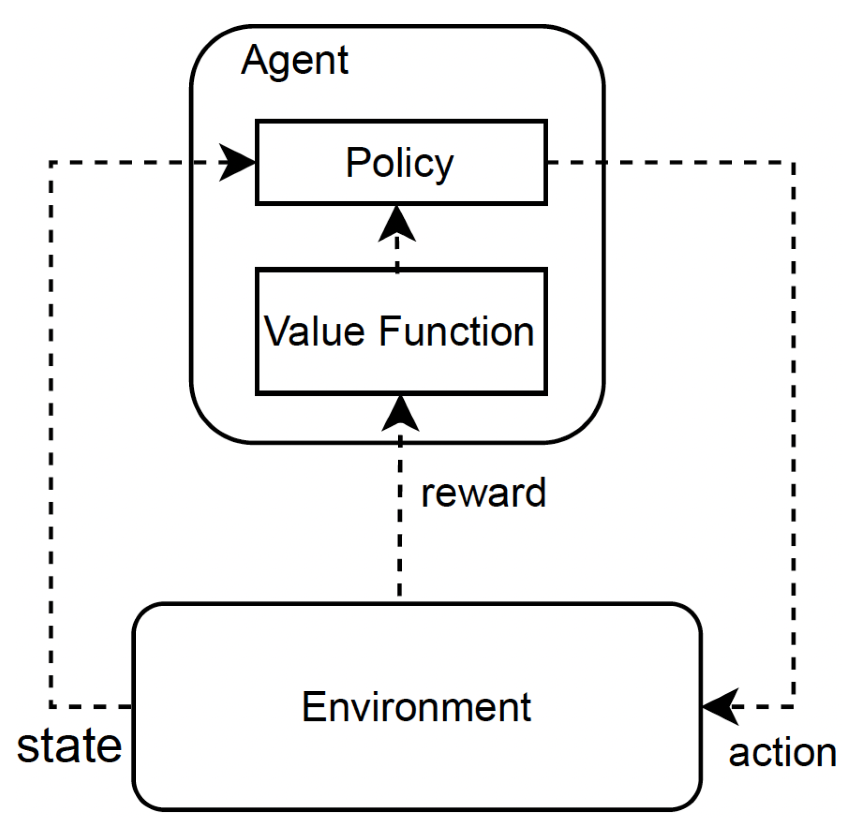
Figure 1. The fundamental operation of the RL mechanism.
Table 1. List of notations.
| Parameters | Labels |
|---|---|
| t | Time step t |
| 𝑠𝑡 | State of the agent at t |
| 𝑎𝑡 | Action of the agent at t |
| 𝑟𝑡 | Reward of the agent at t |
| A | Action space |
| S | State space |
| R | Cumulative reward or return |
| 𝜋 | Policy |
| 𝛽 | Discount factor |
| 𝛼 | Learning rate |
2. State Space
The training of the RL system involves learning from trial and error by interacting with the dynamic environment. The state of the environment plays a crucial role in determining the action taken by the agent. RL models use a state–action pair or an estimated value function that represents the desirability of the current state. In most environments, the state transition follows the Markov property, meaning that the current state 𝑠𝑡 provides sufficient information to make an optimal decision [9]. The model containing state, action, reward, and state transition 𝒯 is referred to as the Markov decision process (MDP). The MDP is a tuple of 〈𝑆,𝐴,𝑇,𝑅〉, in which S is the set of all possible states, A is the set of possible actions, T is the transition function, and R is the reward function. The system is said to be Markovian if the future state of the environment depends only on the current state and the action taken in that state and it is independent of the sequence of states that preceded it.
3. Action Space
The action space refers to the set of all possible actions that an agent can take in a given environment. The agent’s decisions are completely dependent on the environment in which it operates. Thus, different environments result in different action spaces [10]. In some environments, such as Atari and Go, the action space is discrete, meaning that only a finite number of actions are available to the agent [11]. In these cases, the agent must choose one of the available actions at each step. On the other hand, in other environments, such as controlling a robot in a physical world, the action space is continuous [12]. This means the agent can choose an action from a continuous range of values rather than a limited set of options.
4. Reward Function
The reward function, 𝑟(𝑠𝑡,𝑎𝑡), represents the value of taking a particular action, 𝑎𝑡, in a given state, 𝑠𝑡. The goal of the agent is to determine the best policy that maximizes the total reward. The reward function specifies the learning objectives of the agent and is updated at each step based on the new state and action taken.
5. Policy
The policy refers to a strategy or a set of rules that an agent employs to determine its actions in various states of an environment. The policy represents the strategy to map the states to actions. A deterministic policy directly maps states to specific actions, where it provides a probability distribution over actions. The policy is often represented by 𝜋(𝑎|𝑠), where a is an action and s is a state. The optimal policy, 𝜋*, is the one that maximizes the expected cumulative reward received by the agent.
6. State Value and State–Action Value Function
The state value function, denoted as 𝑉𝜋(𝑠), is used to specify the long-term desirability of being in a specific state. On the other hand, the state–action value function, referred to as the Q-function (𝑄𝜋(𝑠,𝑎)), specifies how good it is for an agent to take certain action a in state s under a given policy 𝜋. In Q-learning, the Q-values of state s and action a, i.e., 𝑄(𝑠,𝑎), is determined as follows [13]:

Equation (2) is referred to as Bellman’s equation, in which 𝑄𝜋(𝑠,𝑎) is the Q-value for state s and action a under policy 𝜋, 𝐸𝜋 is the expected value under policy 𝜋, 𝑟𝑡+1 is the immediate reward received, 𝛽 is the discount factor, 𝑠′ and 𝑎′ are the next state and action, respectively, and 𝑠𝑡=𝑠 and 𝑎𝑡=𝑎 are the current state and action.
In addition, the researchers obtain the expected discounted returns for the next potential state–action pair. The update rule for the Q-value function is described as follows:

The values of 𝛼 and 𝛽 are between 0 and 1. The learning rate 𝛼 indicates to what extent new information overrides the previous information. If 𝛼 is 0, the agent learns nothing and relies on previous knowledge only, whereas if 𝛼 is 1, the agent only considers new information irrespective of previous knowledge. Similarly, the discount factor 𝛽 indicates the importance of future rewards. If 𝛽 is 0, that means only the current reward is considered, and if 𝛽 is 1, the agent considers long-term future rewards. The estimated Q-values are stored in a look-up table for each s and a pair. The update rule adjusts the current Q-value estimate based on the observed reward and the maximum expected cumulative reward from the next state. This allows the Q-value estimate to converge towards the true Q-value as more and more experience is gathered.
This entry is adapted from the peer-reviewed paper 10.3390/s23198263
References
- Lindelauf, R. Nuclear Deterrence in the Algorithmic Age: Game Theory Revisited. NL ARMS 2021, 2, 421.
- Moerland, T.M.; Broekens, J.; Plaat, A.; Jonker, C.M. Model-based reinforcement learning: A survey. Found. Trends Mach. Learn. 2023, 16, 1–118.
- Silver, D.; Hubert, T.; Schrittwieser, J.; Antonoglou, I.; Lai, M.; Guez, A.; Lanctot, M.; Sifre, L.; Kumaran, D.; Graepel, T.; et al. Mastering chess and shogi by self-play with a general reinforcement learning algorithm. arXiv 2017, arXiv:1712.01815.
- Mnih, V.; Badia, A.P.; Mirza, M.; Graves, A.; Lillicrap, T.; Harley, T.; Silver, D.; Kavukcuoglu, K. Asynchronous methods for deep reinforcement learning. In Proceedings of the International Conference on Machine Learning, New York, NY, USA, 19–24 June 2016; pp. 1928–1937.
- Schulman, J.; Wolski, F.; Dhariwal, P.; Radford, A.; Klimov, O. Proximal policy optimization algorithms. arXiv 2017, arXiv:1707.06347.
- Lillicrap, T.P.; Hunt, J.J.; Pritzel, A.; Heess, N.; Erez, T.; Tassa, Y.; Silver, D.; Wierstra, D. Continuous control with deep reinforcement learning. arXiv 2015, arXiv:1509.02971.
- Kim, C. Deep reinforcement learning by balancing offline Monte Carlo and online temporal difference use based on environment experiences. Symmetry 2020, 12, 1685.
- Kovári, B.; Hegedüs, F.; Bécsi, T. Design of a reinforcement learning-based lane keeping planning agent for automated vehicles. Appl. Sci. 2020, 10, 7171.
- Mousavi, S.S.; Schukat, M.; Howley, E. Deep reinforcement learning: An overview. In Proceedings of SAI Intelligent Systems Conference (IntelliSys) 2016: Volume 2; Springer: Cham, Switzerland, 2018; pp. 426–440.
- Chandak, Y.; Theocharous, G.; Kostas, J.; Jordan, S.; Thomas, P. Learning action representations for reinforcement learning. In Proceedings of the International Conference on Machine Learning, Long Beach, CA, USA, 9–15 June 2019; pp. 941–950.
- Kanervisto, A.; Scheller, C.; Hautamäki, V. Action space shaping in deep reinforcement learning. In Proceedings of the 2020 IEEE Conference on Games (CoG), Osaka, Japan, 24–27 August 2020; pp. 479–486.
- Kumar, A.; Buckley, T.; Lanier, J.B.; Wang, Q.; Kavelaars, A.; Kuzovkin, I. Offworld gym: Open-access physical robotics environment for real-world reinforcement learning benchmark and research. arXiv 2019, arXiv:1910.08639.
- Clifton, J.; Laber, E. Q-learning: Theory and applications. Annu. Rev. Stat. Its Appl. 2020, 7, 279–301.
This entry is offline, you can click here to edit this entry!