Your browser does not fully support modern features. Please upgrade for a smoother experience.
Please note this is an old version of this entry, which may differ significantly from the current revision.
Subjects:
Transportation Science & Technology
Automotive drive cycles have existed since the 1960s. They started as requirements as being solely used for emissions testing. During the past decade, they became popular with scientists and researchers in the testing of electrochemical vehicles and power devices. They help simulate realistic driving scenarios anywhere from system to component-level design.
- drive cycles
- duty cycles
- drive cycle
- PEMFC
- battery
- hybrid vehicles
- FCHEV
- degradation characterisation
1. Introduction
Drive cycles are standardised speed vs. time data profiles used by automotive manufacturers, testers, and researchers for fuel consumption, emissions, and durability testing and validation [1]. Over the years, they have changed from being used solely for emissions and dynamometer testing in internal combustion engine (ICE) applications to also acting as inputs for vehicle simulations, parameterising, and powertrain component sizing [1]. In a review paper published in 2002 by Esteves-Booth et al., it mentioned simulation and estimation capabilities of certain drive cycles, and how drive cycles provide more than just emissions testing [2]. Over the past decade, battery electric- and fuel cell-powered vehicles have initially attracted more interest and increasingly a higher market share due to a range of legislative and environmental factors. These vehicles have the potential to reduce and, indeed, remove, combustion emissions, including CO2 and NOx, resulting in improved air quality and mitigated environmental impact from personal transportation. When studying the performance of these vehicles or energy sources, drive cycles are a crucial tool to simulate realistic driving. These cycles are used by systems designers and researchers for activities as diverse as cell-level degradation studies to pack-level component sizing.
No global standard exists for drive cycles, although certain drive cycles, such as the Worldwide Harmonised Light Vehicles Test Procedure (WLTP) and Federal Test Procedure (FTP), are extensively employed and becoming mandated to be used by automotive manufacturers upon the release of a new vehicle. Some countries and regions have also implemented their own specific legislative drive cycles, such as The New European Drive Cycle (NEDC) or China Automotive Test Cycle (CATC), while others use a jointly produced worldwide drive cycle [3]. However, all drive cycles have their limitations and are not universally applicable across different vehicle powertrain architectures (ICE, EV, and hybrid), vehicle size classifications, and natures of application. Other limitations have been identified, including not accurately representing real-world driving behaviours, which can include significant differences in energy usage between drive cycles using similar dynamics, locations having different driving dynamics than others, and region-specific driving styles and needs [1,4,5].
Drive cycles can be divided into two categories: modal and transient. Transient drive cycles are usually collected based on real driving data while modal cycles are not.
2. Drive Cycle Classification
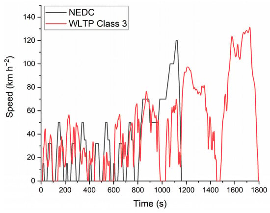
Drive cycles can be divided into two categories: modal and transient [4,5]. Modal drive cycles, such as the New European Drive Cycle (NEDC), are designed for specific regulation testing [1]. Modal drive cycles tend to have sections of linear acceleration and constant velocity, as shown in the NEDC example in Figure 2, and do not accurately depict realistic driving behaviours [1,4,5]. Transient cycles, on the other hand, are collected from real driving data, typically using a global positioning datalogger (GPD) or CAN-BUS readers, such as Advanced Vehicle Location (AVL) [19], OXTS inertial+ [16], or Launch Tech Diagnostic Tools; these tools help determine vehicle location, gradient, and speed data via GPS and CAN messages from a vehicle [1,4,5,20]. Figure 2 is a speed vs. time graphical comparison between a modal (NEDC) and transient (WLTP Class 3) drive cycle. As seen in the figure, modal drive cycles appear less varying, while transient cycles appear more random. NEDC contains four repetitions of the same profile of the ECE-15 drive cycle, which represents urban driving, and one repetition of the Extra-Urban Driving Cycle (EUDC), which represents highway driving. In contrast, the WLTP cycle is divided into four sections: low, medium, high, and extra high. These sections have increasing average speeds to represent driving on distinct types of roads and under different traffic conditions. Low represents congested traffic, medium and high represent more free-flowing urban traffic, and extra-high represents highway driving.
Figure 2. Modal (NEDC) vs. transient (WLTP Class 3) drive cycles. The NEDC drive cycle is a 1180 s modal drive cycle with linear acceleration and constant velocity. It contains two sections: city driving and highway driving. The WLTP drive cycle is a 1800 s transient drive cycle, which represents real-world driving behaviour. Data points are collected by real-world driving. Detailed collection procedures are outlined in the transient drive cycle developmental procedure.
3. Overview and History of Legislative Drive Cycles Sorted by Region and Vehicle Type
3.1. European Drive Cycles
UN-ECE Regulation Number 15 was introduced in Europe, in 1970, to simulate urban driving [11,21]. This modal drive cycle later became a part of the NEDC, which was introduced in 1980 [14,22]. There was legislation regarding vehicle emissions before 1970, in the form of the Agreement of 20 March 1958, which concerned the adoption of uniform conditions of approval and reciprocal recognition of approval for motor vehicle equipment and parts, but no actual drive cycle was introduced [21]. This agreement, however, led to the introduction of UN-ECE Regulation Number 15 in 1970 [21]. The UN-ECE Regulation Number 15 Test consists of three separate parts: Type-I, pollutant emissions testing for speeds up to 50 km h−1; Type-II, carbon-monoxide emissions testing during idling; and Type-III, crank-case emissions testing [11,21]. The regulation was an attempt to evaluate the emissions of urban driving and was later adopted as a component of the New European Drive Cycle (NEDC).
3.2. American Drive Cycles
The US first adopted a modal drive cycle, named ‘California 7-Mode’, in 1968 [7,8]. This drive cycle was mainly based off-road, in Los Angeles, but was used to represent US national driving [7,8]. Even though this drive cycle did not become mandated until 1968, early drive cycle development had been carried out since the 1950s, with the Los Angeles County Air Pollution Control District Laboratory surveying a single Los Angeles route [7,8]. This survey was later updated and improved, in 1956, by the Automobile Manufacturers Association [7,8]. The drive cycle had a duration of only 137 s, with a maximum and average speed of 80 km h−1 and 41.8 km h−1, respectively. As with all modal cycles, this cycle was criticised for not representing real-world driving, especially during rush hour conditions.
In 1972, the US released the EPA Federal Test Procedure for passenger cars, also referred to as the EPA Urban Dynamometer Driving Schedule (UDDS), or FTP-72 [9]. This transient drive cycle was created upon the introduction of the ‘gas guzzler’ tax, which imposed a tax on users with heavy emission vehicles [10]. It has a duration, average speed, and maximum speed of 1372 s, 31.5 km h−1, and 91.3 km h−1, respectively [24].
In 1996, the US Supplemental Federal Test Procedure (SFTP) cycle was developed as an addition to the pre-existing FTP-75 cycle, in the form of SFTP-US06 and SFTP-SC03, to account for higher rates of acceleration, higher speeds, and the use of climate-control functions [25,29]. SFTP-US06 was added to account for higher-velocity driving and has a duration of 596 s, with an average speed and maximum speed of 78 km h−1 and 129 km h−1, respectively [25,30].
Although US SFTP tests were introduced in 1996, they were not mandated until 2007 [29,32]. Specified climate-control test conditions were administered to newly manufactured light-duty vehicles (LDVs) requiring SFTP-SC03 certification [32]. These conditions simulate hot and cold ambient temperatures, i.e., 35 and −7 °C, respectively [32]. Climate-control systems are turned on to represent realistic driver comfort settings, and the vehicle is run on a dynamometer using the SFTP-SC03 cycle [31,32].
3.3. Japanese Drive Cycles
Before the first European and United States legislative cycles were introduced, Japan had developed its driving cycle, the 4-Mode, or J4, in 1966 [34]. The 4-Mode is a simple modal cycle, with cruising speed varying from 10 to 70 km h−1 in increments of 10 km h−1 [7]. 4-Mode has a maximum speed of 70 km h−1 [7]. The Japan 10-Mode replaced this drive cycle in 1973 [7]. Similar to ECE-15, the 10-Mode is a longer driving cycle that simulates urban driving only. Just as EUDC was added to ECE-15 to form NEDC, the 10-Mode was later expanded with a separate drive cycle, named 15-Mode, to represent highway driving, to create a grouped urban and highway driving cycle [7]. The 15-Mode has a top speed of 70 km h−1 [7]. The combination, named the 10–15 Mode, consists of three cycles of 10-Mode and one cycle of 15-Mode. The 10–15 Mode has a duration, average speed, and top speed of 660 s, 22.7 km h−1, and 70 km h−1, respectively [7].
3.4. Chinese Drive Cycles
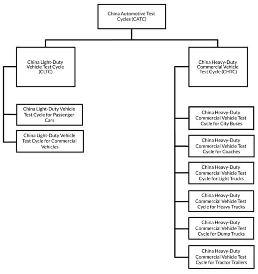
The Chinese Automotive Test Cycles (CATC) were created in 2019 [35,36]; they are divided into light-duty (CLTC) and heavy-duty vehicle (CHTC) tests [36,37]. The tests are further divided according to the specific purposes of these vehicles. The division is shown in Figure 5 [38,39]. This cycle was created based on actual roads in China, using 5000 vehicles that travelled in 41 Chinese cities [37]. A total of 32 million kilometres of data was collected to develop the drive cycle, which is currently the longest sampling distance of all legislative drive cycles. The complete cycle has a duration of 1800 s, an average speed of 28.96 km h−1, and an average acceleration of 0.45 m s−2 [37].
In 2020, the CATC drive cycle became the primary test cycle in China [37]. Before this, WLTP and NEDC were used [38]. CATC was developed in response to the growing concern that NEDC and WLTP did not accurately represent real-world driving behaviour [35,36], given the congested traffic conditions in China. NEDC is a modal cycle that has been widely criticised for its lack of real-world representation.
3.5. Worldwide Drive Cycles—Worldwide Harmonised Light Vehicle Test Procedure (WLTP)
WLTP is the successor to NEDC, which represents a change from a modal cycle to a transient cycle [1,4]. The procedure contains three classes, with each class corresponding to vehicles of different power-to-weight ratios (PWr) [40]. Since September 2017, electric and plug-in hybrid passenger cars in Europe have been required to comply with WLTP for speed requirements; in addition, the emissions testing of LDVs is also performed under this cycle [41,42,43]. This legislation addresses the concern that drive cycles are not only meant to be used as a profile for emissions testing but also as a tool for internal industrial benchmarking.
3.6. Marine Cycles
There is currently no standardised legislative marine cycle. However, this is needed owing to the amount of air pollution caused by fuel oil and liquid natural gas (LNG), marine vehicles, and the need to design and optimise marine vehicles with electric drives. There is a growing concern from residences close to shipping ports experiencing elevated levels of polluted air [45] and the growing use of maritime shipping vehicles. The International Maritime Organisation (IMO) expects a shipping growth of 90 to 130% from 2019 to 2050.
When new marine vehicles are developed, manufacturers tend to use ‘in-house’ drive cycles for a certain proposed water body to help with emissions testing, simulation, and sizing. Most information is inaccessible to the public, so it is difficult to compare and contrast these cycles. An example of an ‘in-house’ public-accessible marine driving cycle is that developed for a public transport boat in Terengganu, Malaysia and explicitly designed for the Kuala Terengganu River [46]. It is a transient cycle developed based on the micro-trip method. Marine drive cycles are also used extensively for military purposes. The US Navy has a drive cycle designed for the DDG-51 Arleigh Burke destroyer ship [47].
Drive cycles and power cycles can be especially useful for PEMFC marine vehicles due to the growing interest in building clean water vehicles and utilising the abundant waterbody nearby to produce hydrogen using electrolysis. The technology is still not mature enough to be fully commercialised; however, various researchers and scientists have deemed the idea to be promising. Power cycles can help determine the possible energy requirements of an estimated trip, which further examines and enhances the usability of having a separate electrolyser onboard the vehicle for ‘live’ hydrogen production.
3.7. Aviation Mission Profile
In the aviation industry, there is a type of testing and simulation data similar to road-vehicle drive cycles, which is typically called a mission profile. Mission profiles focus on categorising aviation movements between engine starts and shut-offs rather than showing numerical speed vs. time data. Some mission profiles can include speed or power data, but this is much rarer compared to the overwhelming amount of road-vehicle speed profiles available for public access. Detailed mission profiles also show altitude vs. displacement data [48,49]. Mission profiles typically start with start-up and taxi out and end with landing and taxi in [49].
4. Comparison of Legislative Drive Cycles
The comparisons only include LDV drive cycles which account for both urban and highway driving, so standalone urban cycles, such as ECE-15, are not included because they will be shown as part of a ‘full’ drive cycle (NEDC contains ECE-15). US legislative drive cycles are also not included, as they are broken down into separate urban and highway driving cycles.
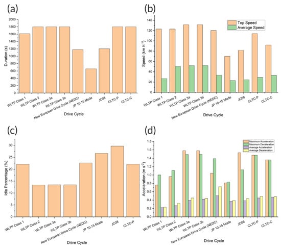
As shown in Figure 7a, the maximum duration of legislative cycles is 1800 s. WLTP (not including Class 1) and CLTP both have the longest duration. Japan has shown relatively shorter durations for both of its drive cycles, even after introducing its transient cycle, JC08. It is a trend to see transient successors of modal cycles having a longer duration.
Figure 7. Comparisons of legislative drive cycles. (a) Duration comparison. (b) Top and average speed comparisons. (c) Idle percentage comparison. (d) Acceleration and deceleration comparisons.
Figure 7b,c show the top speed, average speed, and idling percentage comparisons between legislative drive cycles when also accounting for the idling phases. As shown in Figure 7b, WLTP Class 3 has both the highest top and average speeds. WLTC is representative of many regions throughout the world, where data were collected in the USA, Korea, Japan, India, and various European countries [12].
Both Japanese drive cycles have the slowest top speed; however, as shown in Figure 7c, these cycles also have the highest idling percentage, which is a primary contributor to the low average speed. CLTC cycles have lower average speeds, 17.5 km h−1 lower than that of WLTP Class 3 in the case of CLTC-P, which accurately reflects the more congested road conditions in major Chinese cities [12].
Figure 7d shows a comparison of acceleration and deceleration values for various legislative drive cycles. The comparisons show that transient drive cycles tend to have a higher maximum acceleration than modal ones and are similar to each other in value. For the maximum deceleration, worldwide (WLTP), European (NEDC), and Chinese drive cycles have similar values to one another, regardless of modal or transient. Japanese drive cycles, on the other hand, tend to have less abrupt deceleration. For average acceleration and deceleration comparisons, NEDC has the maximum value for both; while for NEDC’s transient replacement, WLTC, the average deceleration is less abrupt, which better corresponds to real-driving behaviours.
5. Transient Drive Cycle Developmental Procedure Using the Micro-Trip Method
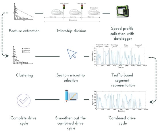
As stated previously, transient drive cycles are based on real-world conditions. Figure 8 outlines the most used transient drive cycle development procedure, using the micro-trips method. To accurately represent driving in the real world, the first step is to collect speed vs. time data with a physical car on real roads, with the aid of a GPS data logger.
Figure 8. Transient drive cycle development procedure using micro-trip clustering technique.
The next stage is micro-trip division. A micro-trip is defined as a discrete period between two points at which the vehicle is immobile or idling [19]. Micro-trips are identified for all speed vs. time profiles collected, creating a series of micro-trips. Depending on the purpose of the drive cycle in development, certain features of each micro-trip (such as average speed or idle percentage) are extracted and plotted onto a two-dimensional scatter plot [19].
After removing the outliers, a set list of traffic conditions is pre-determined (congested urban, urban, extra-urban, and motorway traffic), and the planned duration of each segment can be set [19]. The list may vary depending on the purpose of the drive cycle. This forms the basis of the creation of ‘representative micro-trips’, which means that the collected micro-trips are filtered even further, with several being chosen to represent the pre-determined traffic condition segments [19].
6. Standardised Transient ‘Drive Cycle’ Testing Protocols for Electrochemical Device Testing
Drive cycles (when converted into power cycles) are required to size, design, and optimise powertrains based on electrochemical power sources (and hybrids thereof), including batteries, fuel cells, and supercapacitors. However, there are a lack of pre-converted protocols that can be used. Strictly, drive cycles show speed (km h−1) vs. time (s) data; however, speed is not a relevant parameter when designing electrochemical power systems, which deliver power from current and voltage. Power cycles and current cycles are power vs. time and current vs. time data converted from speed vs. time data, respectively. The Fuel Cells and Hydrogen Joint Undertaking (FCH JU) has a version of the EUDC converted to current vs. time to allow fuel cells to be operated under a drive cycle via current control [13]. However, this is limited to the EUDC cycle, which is a modal cycle and is less representative of realistic driving scenarios compared to transient cycles. There is a lack of publicly available material covering the generation and use of transient power cycles for electrochemical devices. However, there is a commonly used procedure to convert drive cycles to power cycles. This considers the opposing forces of a vehicle, namely aerodynamic drag, rolling resistance, gradient resistance, and gradient force.
7. Drive Cycle to Power Cycle Conversion for Electrochemical Device and Vehicle Testing
Drive cycles started as emissions testing protocols for ICEVs; but, nowadays, they are also crucial for simulation purposes. For example, Ahmadi et al. simulated a PEMFC-battery-supercapacitor electrochemical hybrid vehicle, with FLC EMS under 22 different drive cycles, using the Advanced Vehicle Simulator (ADVISOR) software and analysed the resulting fuel economy and performance using a proposed energy-management strategy [55]. Zhao et al. have studied the trend of resistance changes for a BEV under two different drive cycles using a modelling-based approach [56]. A commonly used degradation testing strategy for fuel cells is the use of accelerated stress tests (AST) and, for batteries, CC-CV charging and CC discharging. However, for a vehicle-based scenario, it is not accurate enough to test electrochemical devices solely using these methods; the implementation of drive cycles can be used to simulate realistic driving behaviour with varying current draw and power requirements at a lab-bench scale. Drive cycles can be converted from speed vs. time units to power vs. time, which can also be called a power cycle, power profile, or duty cycle. Power cycles are important for vehicle and power source modelling, as well as experimental characterisation. This conversion is useful for fuel cell stack or battery pack sizing in an electrochemical powertrain.
8. Using Power Cycles as a Sizing Tool for Electric and Hybrid Vehicles of Different Architectures
The definition of a hybrid vehicle is a vehicle with more than one energy storage system [61]. Currently, most commercially available hybrid vehicles involve hybridising an ICE with a battery pack. However, much research has also gone into electrochemical hybrid vehicles, namely the hybridisation of batteries, fuel cells, and/or supercapacitors. When a power cycle is pre-determined from a theoretical drive cycle, this power cycle can be used for the initial propulsion source sizing of vehicles. Single-power-source vehicles are usually oversized to account for various power losses during a vehicle’s propulsion (transmission losses, aerodynamic drag, and motor losses). However, the source sizing becomes more complicated for hybrid vehicles, as there are more than one energy and power sources to size, and each power unit may experience a vastly different power demand profile from that demanded by the overall vehicle power requirement.
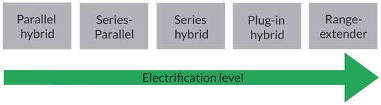
With battery and ICE hybridisation, the battery and ICE component sizing varies depending on the architecture used. Figure 10 shows a ranking of the electrification levels of typical battery-ICE hybrids. In general, the higher the electrification level, the larger the battery needs to be. The same concept can be adapted to all-electrochemical hybrid vehicles. However, instead of the ‘electrification’ level, the classification needs to account for the relative balance between the fuel cell/battery/supercapacitor and the way that they are required to operate together.
Figure 10. Electrification level of battery-ICE vehicles [62,63]. This diagram can also be adapted for electrochemical hybrid vehicles.
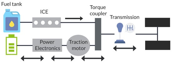
A battery-ICE parallel hybrid vehicle allows the propulsion of the wheels from both the battery and the ICE and is considered as the ‘least electrified’. The battery-electric motor and the ICE are in a parallel layout with a mechanical coupling, hence the name. A typical parallel hybrid architecture is shown in Figure 11. This architecture would typically require a higher-capacity ICE and a smaller-sized battery compared to other systems. The higher engine capacity is to ensure its wheel propulsion capabilities.
Figure 11. Typical parallel architecture. This type of architecture allows propulsion by both the electric motors and ICE [60]. Some manufacturers may steer away from using power electronics to avoid power losses, creating what is known as a passive hybrid system [62].
The same sizing concept can be applied to a parallel fuel cell–battery hybrid architecture. Another sizing consideration that needs to be considered for this hybrid architecture, or any architecture, is whether the system is active or passive. Active systems are hybrid systems with power electronics, such as DC/DC converters, while passive systems are systems without them [64].
For pure BEVs, the sizing chosen for the battery pack should account for both the power and range requirements, in that order. The battery pack needs to be able to fulfil the maximum power requirement of a chosen drive cycle. The number of cells shall then be iterated to increase in a chosen increment until the required range of the vehicle is fulfilled. This initial sizing can be executed in a software-in-the-loop simulation software or programme. Both the power and range requirement should factor in the battery degradation at the end-of-life, as it is likely that the performance of the battery has decreased, particularly in terms of the maximum power drop and capacity fade.
9. Drive Cycles and Duty Cycles for Different Propulsion Systems—Differences, Complications, and Accuracy
Most road vehicles can be divided into three major types of propulsions: internal combustion engine (ICE) propulsion, which commonly requires fuels, such as petrol or diesel; electrochemical propulsion, which utilises batteries, fuel cells, and supercapacitors; and hybrid propulsion, which can be any combination of the above. These different propulsion systems differ in the way that they produce power; and, thus, different sizing strategies of energy sources should be considered when using duty cycles as a required power and energy estimation tool. For ICE vehicles (ICEVs), certain power outputs can only be reached with certain angular velocities, typically measured in revolutions per minute (RPM), and the fuel economy differs when running an engine at different RPMs [67]. ICEV manufacturers typically use engine power and fuel economy vs. engine speed graphs to describe this.
Because of the difference in power delivery patterns of different propulsion sources, manufacturers need to take this into account when using conventional duty cycles as in their sizing calculations; or a propulsion-specific drive cycle needs to be used for that sizing to acquire accurate performance evaluation, optimisation, and range estimation.
Another complication of using power cycles for sizing purposes is the lack of consideration of power or fuel used when the vehicle is stopped (for ICE vehicles, idling). As the conversion of the drive cycle to the power cycle relies on the speed at a given time, the idling power is always considered as zero, which is not realistic. With ICEVs, the engine may still operate during idling, in electrochemical hybrid vehicles, the battery or fuel cell may still be using power. Some vehicles have start–stop technology to prevent this, but there is always some power needed for the vehicle control system and the auxiliary systems, for example, radio systems, infotainment screens, climate-control systems, and alternators.
3. Conclusions
Drive cycles have evolved from being purely emissions testing protocols for ICEVs to tools for vehicle simulation, including electrochemically powered vehicles that use batteries, fuel cells, or supercapacitors. The need to transition the research and development of drive cycle testing from modal to transient and more electric powertrain-suitable drive cycles is crucial. Older modal drive cycles tend to underestimate parameters, such as fuel economy and acceleration, when compared to real-life driving. Modern legislative transient drive cycles for electrochemical vehicles should be developed based on a terrain-to-terrain or driving condition-to-driving condition scenario, suggesting that countries in different regions would require several types of drive cycles. There is no ‘one size fits all’ solution. Certain organisations, such as FCH, have converted drive cycles, such as the EUDC, to be more ‘bench-testing friendly’. However, the protocols still lag behind the intended usage for electrochemical power systems. There are workarounds to the lack of standard testing protocols that simulate realistic driving for these types of vehicles, such as data logging a localised drive cycle or computing a pre-existing drive cycle to a power cycle suitable for rig testing purposes. With the newer advances in electrochemical drive cycles and bench-testing adaptations, various automotive sectors would benefit, including road, marine, and aviation.
This entry is adapted from the peer-reviewed paper 10.3390/en16186552
This entry is offline, you can click here to edit this entry!