Your browser does not fully support modern features. Please upgrade for a smoother experience.
Please note this is an old version of this entry, which may differ significantly from the current revision.
Subjects:
Mathematics, Applied
One of the main challenges faced by iris recognition systems is to be able to work with people in motion, where the sensor is at an increasing distance (more than 1 m) from the person. The ultimate goal is to make the system less and less intrusive and require less cooperation from the person. When this scenario is implemented using a single static sensor, it will be necessary for the sensor to have a wide field of view and for the system to process a large number of frames per second (fps). In such a scenario, many of the captured eye images will not have adequate quality (contrast or resolution).
- eye detection
- iris recognition systems
- Biometric identification
1. Introduction
Biometric identification by iris recognition is based on the analysis of the iris pattern using mathematical techniques. Although it is a relatively recent technique (the first automatic identification system was developed and patented by John Daugman in the last decade of the 20th century), its excellent identification characteristics have led to its rapid evolution. Thus, using the most recent developments, it has become a mature technique. The challenge now is to use it in a scenario where the cooperation of the person is not required to obtain a focused image of the eye but where the person can be allowed to continue walking, keeping the image sensor at a distance of more than 1 m from the person’s face. In iris recognition at a distance (IAAD) systems [1], it is common to use a camera that, thanks to its large field of view (FoV), detects and tracks the face of people approaching the system, and to have several high-resolution iris cameras, with a narrower FoV, that move according to what is determined by the first camera, in order to capture the image that will have the irises to be processed. These systems will therefore employ pan–tilt and control units. As the person is moving, capturing an image of the iris with the appropriate quality in contrast and resolution will require predicting where the person’s face will be at each instant to capture a quality image [2]. However, in cases where the field of view to be covered is not too large, such as an access controlled point, a static system, in which a single high-resolution camera is located, can be used. In this situation, the system shall be able to process these high-resolution images at high speed [3]. The need to capture high-resolution images is imposed by the maintenance of a certain FoV, which would otherwise be too low. On the other hand, having to capture a large number of frames per second is due to the fact that, under normal circumstances, the depth of field of the camera (i.e., the distance around the image plane for which the image sensor is focused [4]) will be very shallow [1]. Because the person to be identified is moving, it is difficult to time the camera shutter release to coincide with the moment when the iris is in the depth of field and therefore in focus. Only by processing many images per second can the system try to ensure that one of the images has captured this moment.
Capturing and pre-processing a large volume of input images requires the use of a powerful edge-computing device. Currently, the options are mainly in the form of graphics processing units (GPUs), application-specific integrated circuits (ASICs), or field-programmable gate arrays (FPGAs). Due to the high power consumption and size of GPUs, and the low flexibility of ASICs, FPGAs are often the most interesting option [5,6]. Moreover, if the traditional development approach of FPGAs using low-level hardware languages (such as Verilog and VHDL) is usually time-consuming and very inefficient, the use of high-level language synthesis (HLS) tools allows developers to program hardware solutions using C/C++ and OpenCL. This significantly improves the efficiency in FPGA developments [7,8]. Finally, FPGAs are nowadays integrated in multi-processor system-on-chips (MPSoC), in which computer and embedded logic elements are combined. These MPSoCs thus offer the acceleration capabilities of the FPGA and the computational capabilities that allow it to work as an independent stand-alone system, which does not have to be connected to an external computer/controller.
2. Embedded Eye Image Defocus Estimation for Iris Biometrics
Defocus blur is the result of an out-of-focus optical imaging system [4]. When an object is not in the focal plane of the camera, the rays associated with it do not converge on the same spot on the sensor but to a region called the circle of confusion (CoC). The CoC can be characterised using a point spread function (PSF), such as Gaussian, defined by a radius/scale parameter [10]. This radius increases as this object gets farther away from the focal plane. In practice, it is assumed that there is a range of distances from the camera, associated with the focal plane, at which an object is considered to be in focus. This is the so-called depth of field of the camera.
The detection of blurred image regions is a relevant task in computer vision. Significantly, defocus blur is considered by several authors to be one of the main sources of degradation in the quality of iris images [2,11,12,13,14]. Many single-image defocus blur estimation approaches have been proposed [4,10]. They can be roughly classified into two categories: edge-based and region-based approaches [10]. The edge-based approach models the blurry edges to estimate a sparse defocus map. Then, the blur information at the edge points can be propagated to the rest of the image to provide a dense blur map [15]. Edge blur estimation models typically consider that the radius of the CoC is roughly constant, and define the edge model using this parameter [16,17]. However, other more complex models of defocused edges can be used [18]. Although edge detection and blur estimation can be performed simultaneously [10], the problem with these approaches is that obtaining the dense defocus map can be a time-consuming step. To alleviate this problem, Chen et al. [16] proposed to divide the image into superpixels, and consider the level of defocus blur in them to be uniform. The method needs a first step in which this division into superpixels is generated. One additional problem with edge-based defocus map estimation is that they usually suffer from textures of the input image [19].
Region-based approaches avoid the propagation procedure to obtain dense defocus maps in edge-based approaches, dividing up the image into patches and providing local defocus blur estimation values. They are free of textures [19]. Some of these approaches work in the frequency domain, as the defocus blur has a frequency response with a known parametric form [20]. Oliveira et al. [21] proposed to assume that the power spectrum of the blurred images is approximately isotropic, with a power-law decay with the spatial frequency. A circular Radon transform was designed to estimate the defocus amount. Zhu et al. [22] proposed to measure the probability of the local defocus scale in the continuous domain, analysing the Fourier spectrum and taking into consideration the smoothness and colour edge information. In the proposal by Ma et al. [23], the power of the high, middle and low frequencies of the Fourier transform is used. Briefly, the ratio of the middle-frequency power to the other frequency powers is estimated. This ratio should be larger for the clear images than for the defocused and motion blurred images. For classifying the images into valid or invalid ones, a support vector machine (SVM) approach is used. In all cases, the approach is simple and fast. These approaches take advantage of the fact that convolution corresponds to a product in the Fourier domain. Also assuming spatially invariant defocus blur, Yan et al. [24] proposed a general regression neural network (GRNN) for defocus blur estimation.
To avoid the computation of the Fourier transform, other researchers prefer to directly work in the image domain. As J.G. Daugman pointed out [25], defocus can be represented, in the image domain, as the convolution of an in-focus image with a PSF of the defocused optics. For simplicity, this function can be modelled as an isotropic Gaussian one, its width being proportional to the degree of defocus [21]. Then, in the Fourier domain, this convolution can be represented as

𝐷𝜎(𝜇,𝜈) and 𝐹(𝜇,𝜈) are the 2D Fourier transforms of the image defocused to degree 𝜎 and the in-focus image, respectively. Significantly, for low (𝜇,𝜈) values, the exponential term approaches unity, and both Fourier transforms are very similar. The effect of defocus is mainly to attenuate the highest frequencies in the image [25]. As the computational complexity of estimating the Fourier transform is relatively high, Daugman suggested to take into consideration Parseval’s theorem
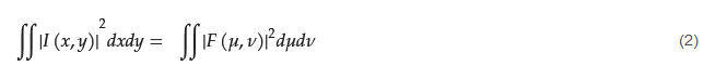
and to not estimate the total power at high frequencies in the Fourier domain but in the image domain. Thus, the idea is to filter the image with a high pass (or a band-pass filtering within a ring of high spatial frequency). After filtering the low-frequency part of the image, the total power in the filtered image is computed using the equation
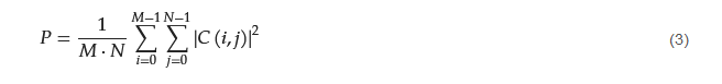
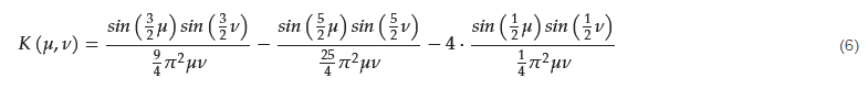
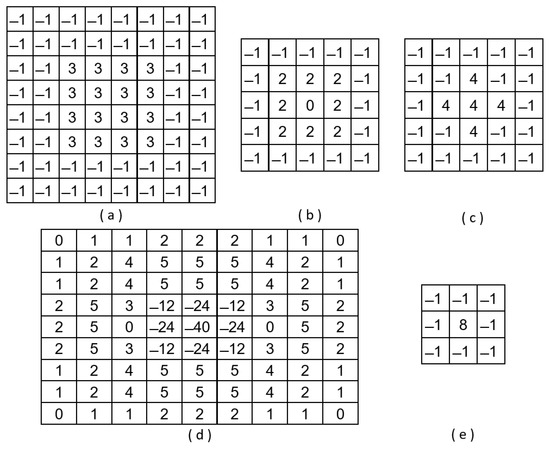
where 𝐶(𝑖,𝑗) is the filtered image of 𝑀×𝑁 dimension. In order to reduce the computational complexity of the Fourier transform, Daugman proposed to obtain the high frequency of the image using a 8 × 8 convolution kernel (Figure 1a). Briefly, this kernel is equivalent to superposing two centred square box functions with a size of 8 × 8 (and amplitude −1) and 4 × 4 (and amplitude +4). The 2D Fourier transform of this kernel can be expressed as the equation
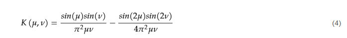
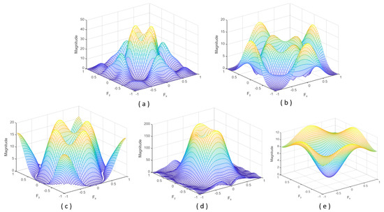
In short, the result is a band-pass filter with a central frequency close to 0.28125 and with a bandwidth of 0.1875. The Fourier spectrum of this kernel is shown in Figure 2a.
It must be noted that, although there is no reference image, to obtain a normalised score between 0 and 100, Daugman proposed that the obtained spectral power x be passed through a compressive non-linearity of the form
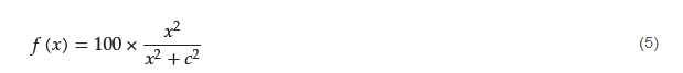
where c is the half power of a focus score corresponding to 50%. This last normalisation step presupposes the existence of a canonical (reference) iris image [26].
Finally, once the signal power value associated with the image (or a sub-image within the image) has been obtained, a threshold value can be set for determining whether the image is clear or out-of-focus [14].
Since, in the scenario, it is possible to assume the isotropic behaviour of the PSF and that the blur is due to bad focusing, this approach based on convolution kernels applied in the image domain is fully valid [21,25]. Furthermore, the convolution filtering of digital images can be efficiently addressed using FPGA devices [7,27,28].
Similar to Daugman’s filter, the proposal by Wei et al. [11] is a band-pass filter, but it selects higher frequencies (central frequency around 0.4375 and a bandwidth of 0.3125). The convolution kernel is shown in Figure 1b. It is a 5 × 5 kernel that superposes three centred square box functions. The frequency response is shown in Figure 2b. Kang and Park [29] also proposed a kernel with a size of 5 × 5 pixels:
This band-pass filter has a central frequency close to 0.2144 and a bandwidth of 0.6076. Thus, the shape of the Fourier spectrum is similar to the one of Daugman’s proposal but with a significantly higher bandwidth (see Figure 2c). Figure 1c shows that it combines three square box functions (one of size 5 × 5 and amplitude −1, one of size 3 × 3 and amplitude +5, and other of size 1 × 1 and amplitude −5).
Since high frequency is associated with sharp changes in intensity, one way to estimate its presence in the image would be to use the Laplacian [30]. The Laplacian 𝐿(𝑥,𝑦)
of an image 𝐼(𝑥,𝑦) is given by 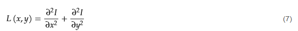
This operator is the basis for the convolution kernel proposed by Wan et al. [30]. To reduce the sensitivity to noise, the Laplacian is applied to an image that is first smoothed by a Gaussian smooth filter. The 2D LoG (Laplacian-of-Gaussian) function has the form
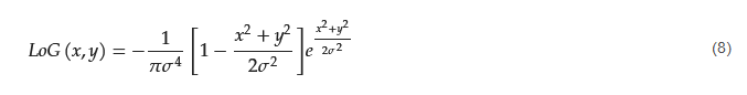
with 𝜎 being the Gaussian standard deviation. For 𝜎 equal to 1.4, the convolution kernel takes the form shown in Figure 1d. The associated Fourier spectrum is illustrated in Figure 2d. However, to simplify the computation, the authors propose an alternative 3 × 3 Laplace operator, combining two square box functions (one of size 3 × 3 and amplitude −1, and other of size 1 × 1 and amplitude +9) (Figure 1e).
This entry is adapted from the peer-reviewed paper 10.3390/s23177491
This entry is offline, you can click here to edit this entry!