A sensor is a detection device that can convert measured data into electrical signals output according to certain rules in order to meet the requirements of information transmission, processing, storage, display, recording, and control [1,2,3]. The performance indicators of sensors usually include sensitivity, resolution, linearity, repeatability, stability, accuracy, and so on [4,5,6]. Sensitivity represents the change in the output of a sensor caused by a change in unit input. It is usually obtained by differentiating the output of the sensor characteristic curve from the input. The higher the sensitivity value, the more sensitive the sensor is. Resolution refers to the ratio between the minimum input increment that a sensor can detect and the full scale, which is used to indicate the minimum measurable input change of the sensor. Linearity represents the degree of deviation between the calibration curve of the sensor and the fitted straight line. The higher the linearity, the smaller the deviation, indicating better sensor performance. Repeatability characterizes the degree of non-coincidence of multiple characteristic curves measured by a sensor under the same working condition when the input is continuously changed multiple times in the same direction. The ideal repeatability error of the sensor should be 0, which means that the curves measured multiple times are completely coincident. Stability refers to the ability of a sensor system to maintain performance for a considerable period, usually expressed as the time difference between the system output and the initial calibration output after a specified time interval at room temperature. The three main indicators that affect stability are time zero drift, zero temperature drift, and sensitivity temperature drift. Accuracy characterizes the maximum deviation between the sensor’s indicated value and the measured true value. From the above indicators, it can be analyzed that all indicators of the sensor cannot be optimal at the same time. For example, sensitivity and stability are contradictory, while high sensitivity indicates low stability, and vice versa. The relationship between resolution and accuracy is that high resolution is a necessary condition for high accuracy, but not a sufficient condition. When selecting a sensor, accuracy should be the first consideration, followed by resolution. In practical applications, because the environment where the sensor located is usually complex, which may be confounding at the same time, and because the signal strength range of the target to be measured is not clear, the selectivity and linear detection range of the sensor must also be taken into account. The good selectivity of the sensor means that it has strong anti-interference ability during operation, and the wide linear detection range means that it can widely receive various signal strengths without causing an overflow.

The intelligent sensor is equipped with a microprocessor to collect, process, and exchange information [7,8,9]. It is the product of the combination of sensor integration and microprocessor. The main distinguishing feature of the intelligent sensor from the general sensor is that it has functions such as self-calibration self-correction, and automatic compensation, as well as the ability to store data and process information [10,11]. Intelligent sensors can correct various deterministic system errors through artificial intelligence, such as nonlinear errors in sensor input and output, server error, zero-point error, forward and backward stroke error, etc., and can also appropriately compensate for random errors and reduce noise, greatly improving sensor accuracy [12,13,14]. In addition, the miniaturization of intelligent sensor systems eliminates some unreliable factors of traditional structures, improves the anti-interference performance of the entire system, and has good stability. Finally, intelligent sensors can achieve comprehensive measurement of multiple sensors and parameters and can expand the measurement and usage range through programming, with certain adaptive capabilities. Its digital communication interface function can directly send data to terminals of various application systems for processing. Regardless of the type of sensor, the electrical signal output by their conversion elements is generally weak and accompanied by noise. Therefore, before signal acquisition, a signal conditioning circuit is required to amplify and filter the signal. The interface circuit further processes the electrical signal to produce an output consistent with the use of a measurement or control system [15,16,17]. In the end, the output electrical signal becomes a digital signal after analog-to-digital, and the control system resolves the state of the measured amount from the digital signal and views it through the communication or uses it directly for regulation.

In summary, the construction of intelligent sensors requires three elements: sensitive components, interface circuits, and communication interfaces. Since microprocessors are already mentioned in the definition of intelligent sensor sensors, they are not listed here as necessary elements. As the medium of signal type conversion, the selection of sensitive elements is particularly important, which directly affects the performance parameters of the whole sensor, such as signal-to-noise ratio, resolving power, accuracy, etc. Typically, the sensitive element is more dependent on the environment. Changes in temperature, humidity, light intensity, and other environmental factors may cause instability of the sensitive element [18,19]. The self-calibration function of intelligent sensors before working makes them more widely used than ordinary sensors. It is necessary to emphasize that the calibration of a sensor relies on a known calibration signal and the calibration process will inevitably generate errors that affect sensor accuracy [20]. Nevertheless, the sensor still needs to be calibrated after a certain period. Interface circuits are often defined as processing circuits for the output signals of sensitive components, which include impedance conversion circuit, amplifier circuit, current-voltage conversion circuit, bridge circuit, frequency-voltage conversion circuit, charge amplifier circuit, filter circuit, etc.

The process of experimentally determining, under predetermined measurement conditions, the correspondence between a sensor’s input and output is known as calibration. The sensor has to be recalibrated if any of its indicators have changed as a result of the external environment or if it has been some time since the last calibration. Usually, the sensor is calibrated once in the factory and then again according to user requirements. All sensors require calibration in order to function normally since it is the only way for the sensor to obtain calibration equations and because it establishes the accuracy of the sensor’s analog signal output.

The basic method of calibration is to input a known signal to the sensor and obtain the output signal at the same time, thus obtaining a series of curves characterizing the correspondence between the two. In all calibration results, the linear relationship is undoubtedly the simplest and most conducive to sensor calibration. When the calibration result is non-linear, a reasonable data processing method is usually selected to linearize it. When calibrating sensors, the accuracy of the measuring equipment used is usually an order of magnitude higher than that of the sensor to be calibrated for error minimization calibration. Specifically for a piezoelectric pressure sensor, a piston manometer is used to generate a standard force of known magnitude on the sensor, which will output a corresponding charge signal, which is then measured by a standard detection device of known accuracy to obtain the magnitude of the charge signal, resulting in a set of input-output relationships. The relationship can generally be described by an equation whose parameters are referred to as calibration factors. Such a series of processes is the calibration process for piezoelectric pressure sensors.

For the purpose of ensuring measurement accuracy, self-calibrating sensors employ a variety of technical techniques to remove drift. In some ways, self-calibration is the same as recalibration prior to every measurement, which can remove the sensor system’s drift in temperature and time. This requires the integration of the corresponding calibration signal source as well as the calibration control circuit or algorithm in the sensing system. If the calibration signal source cannot be integrated into the system, it can only be obtained from an external source, which improves calibration accuracy but is less convenient. The calibration control circuit includes cross-sensitivity compensation, differential compensation, background calibration, etc. In summary, the self-calibration of the intelligent sensor is a process of automatically collaborating with the microcontroller and actuator to calibrate sensor components. Although self-calibration cannot completely take the place of an actual calibration, it may reduce the number of calibration points required for a given accuracy condition or extend the time between calibrations. The information storage capacity of intelligent sensors is the basis for successfully accessing the chain of calibration during self-calibration. The intelligent sensor saves calibration data in an electrically erasable programmable read-only memory (EEPROM) during calibration, which can be recalled by the microprocessor at any time when it is needed. EEPROM is generally a separate integrated chip that can be used “plug-and-play” on the same sensor, which means that the relevant calibration data does not need to be updated separately when replacing or recalibrating the same intelligent sensor.

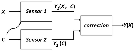
Figure 1 shows the principle of cross-sensitivity compensation, where both the interference signal C and the signal to be measured X can cause a change in the output signal of sensor 1. To eliminate the influence of the interference signal C, the cross-sensitivity is compensated for by the detection of the interference signal C by sensor 2. The effectiveness of this method depends on the reproducibility of the cross-sensitivity of sensor 1 to the interfering signal C [23]. If this cross-sensitivity is highly variable over time, then the improvements that can be obtained may be limited. Where sensors have a defined cross-sensitivity, the addition of sensors can significantly improve overall performance.

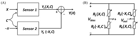
Differential compensation in which two identical sensors are used to measure two signals of the same magnitude and opposite phase that are to be measured (Figure 2A). As the interfering signal C acts on both sensors simultaneously, the resulting errors are canceled out in the subsequent calculation. Figure 2B shows an example of a typical differential compensation circuit called the Wheatstone full-bridge [24]. R1 and R2 are shown as a set of strain gauges placed perpendicular to each other, as are R3 and R4. The changes caused by temperature on the four strain gauges should be the same and the absolute value of the change in resistance of the four strain gauges should be the same when the object is deformed. A simple calculation shows that the final output voltage Vout is proportional to the absolute value of the change in resistance [25]. There is no non-linear error and the sensitivity is numerically equal to the supply voltage Vbias.

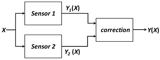
Background calibration is the use of two different sensors to measure the same signal, as shown in Figure 3. The two sensors have different characteristics: for example, one of them is more accurate but has a slow response time, and the other one is less accurate but has a fast response time. In this case, the system often compares the data from the two sensors and corrects the output with a faster response. The combination of these two sensors produces a fast and accurate measurement system.