1. Introduction

Natural systems in the physical world undergo constant change due to driving forces such as thermal variation, solar insolation level and chemical reactions. The paper examines solar cycles 21 to 25 up to 2010. Generally, sunspot activity follows an 11-year periodic oscillation with some chaotic tendencies. A single predictive equation would enable look-ahead modelling allowing society to prepare for peaks and toughs in temperatures and their associated affects.

Modelling solar cycles is achieved using a modified logistic map. Euler developed the basis of numerous mathematical techniques [1]. Coupled with a growth curve given by Verhulst, a new combination difference equation is formulated that describes growth-limited trajectories and solar cycles [2].

Interest in sunspot count and solar cycles exist due to their effect on the earth’s environment which include heating, radiation levels and insolation. Typically, sunspot count peaks between 100 and 300 in any cycle. Solar cycle prediction requires a method that models long-term periodicity and sunspot count amplitude.

2. Methods and Application

2.1. Difference Equation Development

Euler’s expansion of any function N(t) generates discrete values separated by a time step interval δ = () producing discrete values with β an introduced gain parameter. Upper-limit growth of the Verhulst logistic equation may be substituted for the derivative in the Euler expansion, forming a new discrete domain equation with a delay,

and by adding a new modulation function m(T) gives the complete difference equation 

,                                                 (1)

λ being the growth parameter, k = -1, ε = 1/P, P is the upper limit or target growth value, γ = (β + λ) and ρ = λ/P. A delay term φ in the growth-limited part of the logistic equation produces chaotic solutions that are often only stable over a very narrow range of parameters [4]. Term  forms a modulation function with an approximate 50-year sunspot peak-to-trough interval, defined by . Individual growth and decay curves may be coupled as a difference pair to emulate a pulse-like curve,

                                                   (2a)

                                                 (2b)

where Nf and Nr describe the rise and fall of a discrete count, respectively. A single pulse curve may be generated by taking the product of the recursion results above,

                                                                  (3)

2.2. Single Solar Cycle Model

Galactic activity such as solar cycles or sunspot count over an 11-year period are amenable to recursive modelling for multiple solar cycles using equation (1), or to individual cycle pulse shape modelling by equations (3). Figure 1(a) shows sunspot count during solar cycle 21 (1976-1987), compared to recorded data [3]. Examination of the sunspot count for each year in solar cycle 21 shows that equation-pair (2-a) and (2-b) applied to equation (3) form a piece-wise correlation describing solar cycle 21 pulse shape according to equation (3).

Initial condition for equation (2-a) are λ = 1.3, ε = 1/250 and Nr (T=0) = 23, rising towards 250 over the discrete range (years) 0 < T < 12. The simulated curve for equation (2-a) is shown on Figure (1a) by the left-side dashed curve. Initial conditions for used for equation (2-b) are Nf (T=0) = 250, falling towards zero over the same discrete range 0 < T < 12. The result is plotted in the right-side dashed curve of Figure 1(a). The combined product curve using equation (3) closely matches sunspot data.

2.2. Multiple Solar Cycle Model

Figure 1(b) shows the application of equation (1) to model multiple solar cycles 22, 23 and part of solar cycle 24 up to 2014. Initial conditions for stability use kφ = -2, γ = 1.75, λ = 1.5, ρ = 1.5/P, P = 210 and = 40.05 in equation (1). The term  represents a double delay in the recursion.

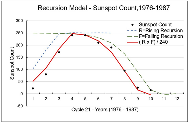
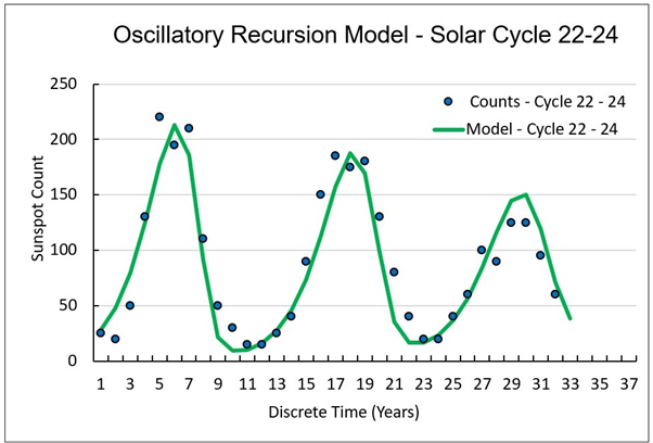
Figure 1. Reported sunspot cycle count in relation to recursive solutions: (a) Piece-wise application of equations (2-a) and (2-b), showing a graph of their product; (b) Delay equation (1) simulating oscillations in sunspot count over two full cycles, compared to reported measurements.

3. Discussion and Concluding Comments

Peak sunspot counts for solar cycles 22, 23 and 24 became progressively lower by 40 counts over the last 33 years. Stability of the oscillations generated by equation (1) are marginal and dependent on a very narrow band of parameter selections. Of interest to dynamics in the natural sciences is the development of a single equation defining a trajectory that compares to recorded data sets in the discrete time domain. Sunspot count is generally predicable over an 11-year period, and analysis shows that a general expression describes the sunspot count numbers. In solar cycle 21 the peak count recorded by various institutions was near 240. During the last two cycles, peaks reached 200 counts, and the last cycle 24 a peaked at 130 in 2014.

In general, the shape of a growth/decay recursion curve is parametrically adjustable, providing a method for describing discrete data sets by a single recursion equation. Curves generated by recursion are not related to regression curve fitting, and have the added advantage that forward predictions can be made in the discrete time domain based on a few initial conditions and data points. A full research paper on this subject would naturally expand on back-predictive recursions to enable confidence in the forward solar cycle activity for the next 50 years.

References

1. Lokoba, T.I. Simple Euler method and its modifications. In Lecture Notes Math 337, University of Vermont, USA, 2012, pp. 6-14.
2. Verhulst, P.F. Recherches mathematiques sur la loi d’accroissement de la population. Mem. De l’Academie Royale des Sci. et Belles-Lettre de Bruxxelle 1845, 18, 1-41.
3. justinweather.com/2018/10/29/sun-spot-cycle-solar-minimum-often-means-more-winter-snow/
4. Lisena, B. Periodic solutions of logistic equations with time delay. Math. Lett 2007, 20, 1070-1074