Reinforcement Learning | Encyclopedia MDPI

Reinforcement Learning: History

Please note this is an old version of this entry, which may differ significantly from the current revision.

Contributor:

Reinforcement Learning (RL) is an approach in Machine Learning that aims to solve dynamic and complex problems, in which autonomous entities, called agents, are trained to take actions that will lead them to an optimal solution

Reinforcement Learning (RL)
Hierarchical Reinforcement Learning (HRL)
Machine Learning
deep learning

1. Introduction

Reinforcement Learning (RL) portrays a promising control approach for energy system optimization owing to its capability to learn from past encounters and adapt to changing system dynamics. RL can handle the complexity and uncertainty of energy systems and develop optimal control policies that maximize performance metrics such as energy efficiency, cost savings and reduced carbon emissions. There are two primary types of RL: model-based and model-free. In model-based RL, the agent has a model of the environment, which is used to simulate the effects of different actions. The agent can then choose actions that maximize a long-term reward function. Model-based RL is similar to Model Predictive Control (MPC) in that both involve a model of the system and use it to predict the effects of different actions and control scenarios ^[1]^[2]. It should be noted though that model-based RL is focused on maximizing a long-term reward, while MPC is focused on minimizing a cost function over a finite horizon. Additionally, model-based RL is more flexible and adaptable to system alterations, while MPC assumes a static environment and may require returning if significant changes occur. On the other hand, model-free RL methodologies present a model-independent nature—thus, they do not require the generation of an accurate mathematical model of the system being controlled, which can be difficult to develop and maintain for complex energy systems.

The agents learn to make optimal decisions as they exist in an environment and interact with it over time. The learning process is accomplished through a trial-and-error approach, as the agent’s actions are taken after receiving feedback from the environment, in the form of a reward or penalty, for their previous action. The basic structure of RL can be seen in Figure 1, where an agent outputs an action and receives the new environment state and its reward, at timestep t. Finding the optimal solution should ultimately lead to the maximization of a cumulative reward over time, commonly referred to as the agent’s return.

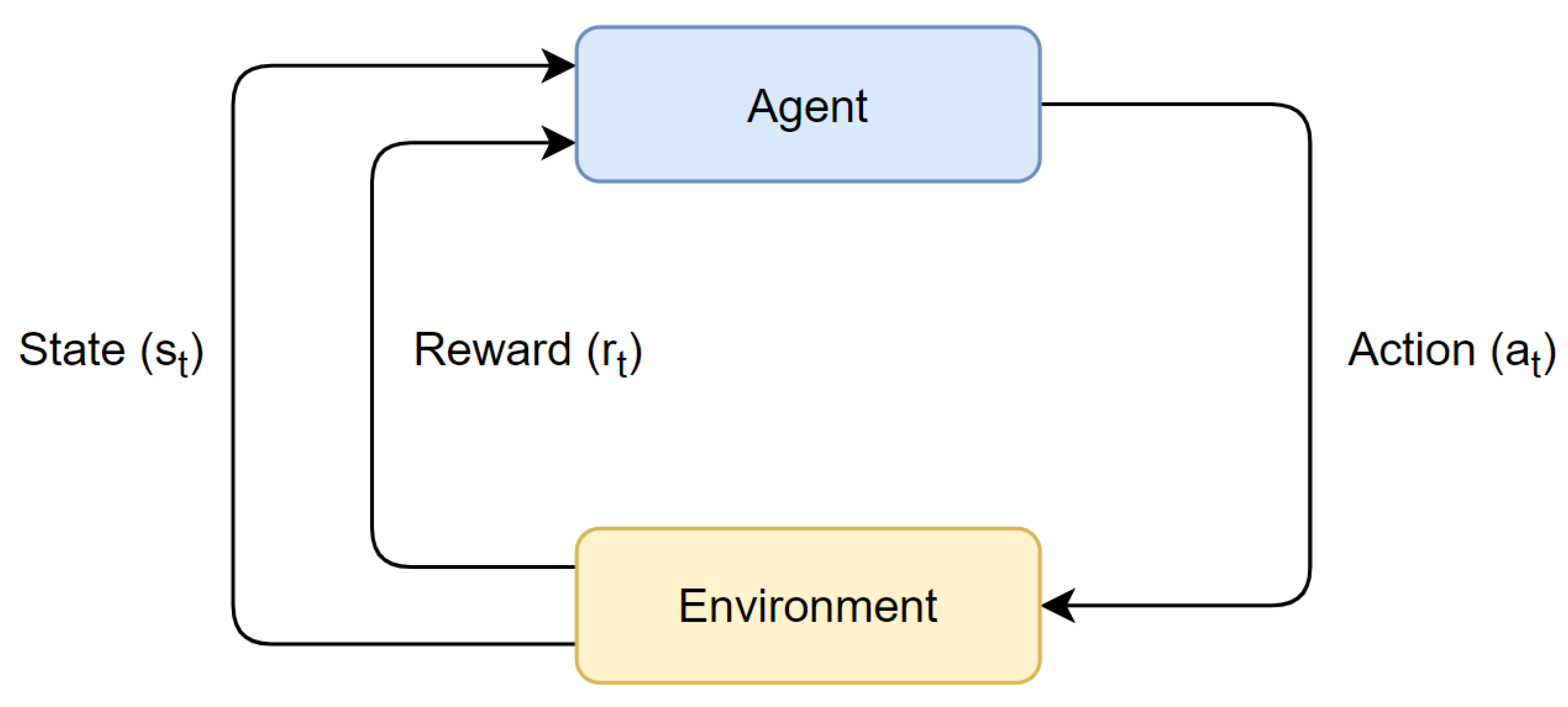
Figure 1. The Reinforcement Learning Framework.

2. Markov Decision Processes

The general mathematical formulation of the RL problem is a Markov Decision Process (MDP). An MDP is a mathematical model that describes the interaction between the agent and the environment. It follows the Markov Property, which states that the conditional probability distribution of future states of a stochastic process depends only on the current state and not the previous ones. This means that the history of previous states and their actions’ consequences do not define the future states. The Markov Property is the basis for the mathematical framework of Markov models, which are widely used in a variety of fields, including physics, economics and computer science. MDPs describe fully observable RL environments and they consist of a finite number of discrete states. The agent’s actions cause the environment to transition from one state to the next and the goal is to discover a policy that is associated with an action to maximize the expected cumulative reward or return, over time.

An MDP can be described by the tuple (

S, A, P, R, ρ_{0}, γ, π

), where:

$S$ denotes the state space, which contains all the possible states an agent can find itself in;

$A$ denotes the action space, which contains all the possible actions an agent can take;
$P$ denotes the transition probability of the agent, $P (s_{t + 1} | s_{t}, a_{t}$ ), where $t + 1$ is the next time step and t the current one;

$R (s_{t}, a_{t}$ ) denotes the reward function which defines the reward the agent will receive;
$ρ_{0}$ denotes the start-state distribution;
$γ \in [0, 1)$ denotes the discount factor, which determines the influence an action has in future rewards, with values closer to 1 having greater impact;
$π (a | s)$ is the policy which maps the states to the actions taken.

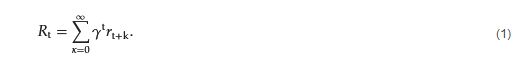
In RL algorithms, the agent interacts with its environment in timesteps

t = 1, 2, 3, \dots

In each timestep the agent receives an observation of the environment state,

s_{t} \in S

and then chooses an action,

a_{t} \in A

. In timestep

t + 1

, the agent will receive the arithmetic reward,

r_{t} \in R \subset ℜ

, for the action taken. The policy in an MDP problem gives the probability to transition to state s when executing action a. The main objective in an MDP problem is to find an optimal policy,

π *

, which ultimately leads to the maximization of the cumulative reward, given by Equation (1).

3. Value Functions and Bellman Equations

In the RL framework, value functions have a critical role in estimating the expected cumulative reward that an agent will receive if it follows a particular policy and starts its course of action from a specific state or a state–action pair ^[3]^[4]. A fundamental distinction between value functions and reward functions is that the latter provide immediate rewards to the agent, according to its most recent action, whereas the former estimate cumulative rewards in the long term. Thus, the value function estimates the expected sum of rewards that an agent will obtain from a specific state over the entire duration of its interaction with the environment. This makes the value functions difficult to estimate, given that the value of a state or state–action pair must be estimated multiple times throughout an episode from state observations recorded during an agent’s lifetime. Bellman Equations are mathematical expressions utilized for the purpose of computing the value functions in an efficient, recursive way. Specifically, the Bellman Equation expresses the value of a state or state–action pair as the sum of the immediate reward received in that state and the expected value of the next state under the policy being followed by the agent ^[3]. The Bellman Equation takes into account that the optimal value of a state is dependent on the optimal values of its neighboring states and it iteratively estimates and updates the value functions and the policy followed. This iterative process is repeated until the value functions converge to their optimal values and therefore reach the optimal policy. When the agent initiates its actions from a specific state, the value function is referred to as the ‘state-value’ function, whereas when the agent initiates from a specific state–action pair, it is then called the ‘action-value’ function. The state value describes the expected performance of an agent, when it follows policy

π

and has started from state s. The mathematical representation of a typical value function is as seen in Equation (2), while the Bellman Equation for the value function which expresses the dependency of the value of one state with the values of future states is seen in Equation (3).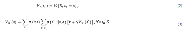

Respectively, the action-value describes the expected performance of an agent when it chooses action a, while it finds itself in state s and follows policy

π

. Then, the mathematical representation of the value function is as in Equation (4) and the Bellman equivalent is as in Equation (5).

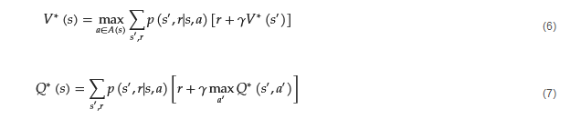
This equation is also known as the Q-function, which calculates the Q-value or ’quality value’, of the RL agent. These equations have their optimal equivalents, in which the policies followed are the optimal policies of the agent. The optimal equations, which are given by Equations (6) and (7), are called ’Bellman Optimality Equations’ and describe the optimal action-value function in terms of the optimal value function. These equations in reality describe a system of equations, with each equation corresponding to one state.

4. Reinforcement Learning Methods and Algorithms

The RL methods can be divided into two categories: model-based and model-free methods ^[4]. In model-based methods, there is a model which mimics the behavior of an environment and has the ability to observe a state and action and immediately determine the reward of the agent and the future state. The agent utilizes the model in such a way that it can simulate different sequences of actions and predict their outcomes. These methods can achieve faster learning as the model of the system is built beforehand. It can also provide higher sample efficiency, as it leads to the accurate generation of additional training data to improve the agent’s performance. In model-free methods, the agent is trained effectively in complex and unknown environments, as it learns directly from the previous experience the agent has gathered. A model which could be inaccurate and lead to potentially unwanted results does not exist; therefore, the agent needs to rely solely on the trial-and-error approach. Model-free and model-based RL methods can, in turn, be divided into two more categories, policy optimization and Q-Learning, also known as policy-based and value-based methods, and learn the model given the model methods. This entry will focus on model-free methods and their subcategories, as the main advantages of RL are modeling and environment agnostic approaches. In conclusion of this section, a comprehensive table is presented, showcasing state-of-the-art RL algorithms. The classification of these algorithms is based on their respective approaches to policy optimization, Q-learning, or a combination of both (see Table 1).

4.1. Policy-Optimization and Policy-Based Approaches

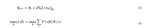
Policy-optimization methods directly update the agent’s policy and their objective is to discover the optimal policy, which will lead to the maximization of the expected cumulative reward, without explicitly learning a value function. They use stochastic policies,

π_{θ} (a | s)

, and attempt to optimize the

θ

parameters of the policy through various techniques. One technique is the gradient ascent technique, which aims to find the maximum of an optimality function

J (π_{θ})

, as seen in Equation (8). Another technique is the maximization of local estimates of this function, as seen in Equation (9). Gradient-based policy-optimization algorithms are known as policy gradient methods, as they directly compute the gradient,

\nabla_{θ} J (π_{θ})

, of the expected cumulative reward in terms of the policy parameters and use this gradient to compute the policy. Policy gradient algorithms are mostly on-policy methods, as in every iteration data gathered from the most recent policy followed is used. They can learn stochastic policies, which can be useful in environments with uncertainty; they can handle continuous action spaces and learn policies that are robust to environments with uncertainty.

Policy-optimization methods also include techniques that introduce a constraint to ensure policy changes are not too large and maintain a certain level of performance. These are called trust region-optimization methods. Additionally, policy gradient algorithms include actor–critic methods, which consist of two components: the actor-network, or the policy function, responsible for the choosing of the agent’s action, and the critic network, or the value function estimator, responsible for the estimation of the value of state–action pairs. The actor receives the critic’s estimate and proceeds to update its policy with respect to the policy parameters. Actor–critic methods leverage the benefits of both value-based and policy-based methods. Some of the most well-known policy-optimization methods are Proximal Policy Optimization (PPO) ^[5], Trust Region Policy Optimization (TRPO) ^[6], Vanilla Policy Gradient (VPG) ^[7], Deep Deterministic Policy Gradient (DDPG) ^[8], Soft Actor–Critic (SAC) ^[9], Advantage Actor–Critic (A2C) ^[10] and Asynchronous Advantage Actor–Critic (A3C) ^[10].

4.2. Q-Learning and Value-Based Approaches

Q-Learning methods ^[11]^[12] are characterized as off-policy learning methods that do not require a learning model, where the agent learns an action-value function, the Q-function,

Q_{θ} (s, a)

, for the optimal action-value function,

Q_{*} (s, a)

. This function estimates the expected return of selecting action a, in state s, and following the optimal policy from the next state, s′. The Q-function’s objective is to maximize quality values of a state, the Q-values, by choosing the appropriate actions for each given state. It simultaneously updates the Q-values of that state. The Q-function is given by Equation (10).

The best actions of the agent for a state, s, are selected through a greedy method, called

ϵ

-Greedy. The selection of these actions happen with a probability

1 - ϵ

, while the selection of a random future action happens with a probability of

ϵ

, where

ϵ \in (0, 1)

The

ϵ

-Greedy method is an approach to the exploitation versus exploration problem, where the agent needs to find an equilibrium between exploiting the selection of previously found good actions which yield satisfying rewards and exploring new and potentially better, unknown actions. Q-Learning techniques are characterized by their simplicity and ease of implementation. They are utilized in continuous and discrete state and action spaces and have the ability to learn from experiences that do not have an optimal policy. Some well-known extensions and improved methods that are derived from Q-Learning are Double Q-Learning ^[13], Deep Q-Networks (DQNs) ^[14] and Dueling Q-Learning ^[15]. Double Q-Learning attempts to solve the problem of overestimation of Q-values in certain scenarios by modifying the original Q-Learning algorithm and learning two Q-functions independently as estimators. The Q-function that yields the highest Q-value is the primary estimator whose Q-value will be selected. The other Q-function is the secondary estimator used to estimate the Q-value of the selected action, which helps reduce the overestimation bias that can occur in standard Q-Learning. DQNs make use of deep neural networks which take the current state as input and outputs the estimated Q-value of the Q-function. This is achieved by updating the weights of the network and minimizing the mean squared error between the predicted and actual Q-values. Dueling Q-Learning makes use of a state-value function, which estimates the value of a particular state and an advantage function, which estimates the advantage of taking an action in that state. The Q-value is the sum of the advantage and state-value functions, minus the mean of the advantage of all previous actions.

Table 1. State-of-the-art RL algorithms.

Policy Optimization	Q-Learning	Policy Optimization and Q-Learning-Based
Vanilla Policy Gradient ^[7]	Double Q-Learning ^[13]	DDPG ^[8]
PPO ^[5]	DQN ^[14]	SAC ^[9]
A2C/A3C ^[10]	Dueling Q-Learning ^[15]	TD3 ^[16]
TRPO ^[6]	C51 ^[17]

This entry is adapted from the peer-reviewed paper 10.3390/en16145326

References

Moerland, T.M.; Broekens, J.; Plaat, A.; Jonker, C.M. Model-based Reinforcement Learning: A survey. Found. Trends® Mach. Learn. 2023, 16, 1–118.
Pong, V.; Gu, S.; Dalal, M.; Levine, S. Temporal difference models: Model-free Deep RL for model-based control. arXiv 2018, arXiv:1802.09081.
Sutton, R.S.; Barto, A.G. Reinforcement Learning: An Introduction, 2nd ed.; MIT Press: Cambridge, MA, USA, 2018.
Wiering, M.; Otterlo, M.v. Reinforcement Learning: State-of-the-Art; Springer: Berlin/Heidelberg, Germany, 2012.
Schulman, J.; Wolski, F.; Dhariwal, P.; Radford, A.; Klimov, O. Proximal Policy Optimization Algorithms. arXiv 2017, arXiv:1707.06347.
Schulman, J.; Levine, S.; Abbeel, P.; Jordan, M.; Moritz, P. Trust Region Policy Optimization. In Proceedings of the 32nd International Conference on Machine Learning, Lille, France, 7–9 July 2015; Volume 37, pp. 1889–1897.
Sutton, R.S.; McAllester, D.; Singh, S.; Mansour, Y. Policy Gradient Methods for Reinforcement Learning with Function Approximation. In Advances in Neural Information Processing Systems; Solla, S., Leen, T., Müller, K., Eds.; MIT Press: Cambridge, MA, USA, 1999; Volume 12.
Lillicrap, T.P.; Hunt, J.J.; Pritzel, A.; Heess, N.M.O.; Erez, T.; Tassa, Y.; Silver, D.; Wierstra, D. Continuous control with deep Reinforcement Learning. arXiv 2015, arXiv:1509.02971.
Haarnoja, T.; Zhou, A.; Abbeel, P.; Levine, S. Soft Actor–Critic: Off-Policy Maximum Entropy Deep Reinforcement Learning with a Stochastic Actor. In Proceedings of the 35th International Conference on Machine Learning, Stockholm, Sweden, 10–15 July 2018; Volume 80, pp. 1861–1870.
Mnih, V.; Badia, A.P.; Mirza, M.; Graves, A.; Lillicrap, T.; Harley, T.; Silver, D.; Kavukcuoglu, K. Asynchronous Methods for Deep Reinforcement Learning. In Proceedings of the 33rd International Conference on Machine Learning, New York, NY, USA, 20–22 June 2016; Volume 48, pp. 1928–1937.
Watkins, C. Learning from Delayed Rewards. Ph.D. Thesis, King’s College, London, UK, 1989.
Watkins, C.; Dayan, P. Q-Learning. Mach. Learn. 1992, 8, 279–292.
Hasselt, H. Double Q-Learning. In Advances in Neural Information Processing Systems; Lafferty, J., Williams, C., Shawe-Taylor, J., Zemel, R., Culotta, A., Eds.; Curran Associates, Inc.: Red Hook, NY, USA, 2010; Volume 23.
Mnih, V.; Kavukcuoglu, K.; Silver, D.; Rusu, A.A.; Veness, J.; Bellemare, M.G.; Graves, A.; Riedmiller, M.A.; Fidjeland, A.K.; Ostrovski, G.; et al. Human-level control through deep Reinforcement Learning. Nature 2015, 518, 529–533.
Wang, Z.; Schaul, T.; Hessel, M.; Hasselt, H.; Lanctot, M.; Freitas, N. Dueling Network Architectures for Deep Reinforcement Learning. In Proceedings of the 33rd International Conference on Machine Learning, New York, NY, USA, 20–22 June 2016; Volume 48, pp. 1995–2003.
Fujimoto, S.; van Hoof, H.; Meger, D. Addressing Function Approximation Error in Actor–Critic Methods. arXiv 2018, arXiv:1802.09477.
Bellemare, M.G.; Dabney, W.; Munos, R. A Distributional Perspective on Reinforcement Learning. arXiv 2017, arXiv:1707.06887.

© Text is available under the terms and conditions of the Creative Commons Attribution (CC BY) license; additional terms may apply. By using this site, you agree to the Terms and Conditions and Privacy Policy.