Your browser does not fully support modern features. Please upgrade for a smoother experience.
Please note this is an old version of this entry, which may differ significantly from the current revision.
A two-stage framework based on the distribution propagation graph neural network (DPGN) called the multilevel distribution propagation network (MDPN). An instance-segmentation-based object localization (ISOL) module and a graph-based multilevel distribution propagation (GMDP) module are both included in the MDPN.
- deep learning
- few-shot classification
- graph neural network
1. Introduction
A significant amount of labeled data is needed for traditional deep-learning techniques. However, there are times when there are very few samples accessible because of the security, morality, resource, and expense concerns associated with data collection. Few-shot learning (FSL) was used to find a solution to this issue. FSL seeks to develop models that perform well when trained on small-scale data. Additionally, FSL can significantly lower the cost of manual annotation and has a broad range of potential applications in data-scarce areas such as uncommon disease data and human-computer interaction.
However, the backbone can only be set up as a lightweight network with shallow depth and narrow width, such as ConvNet4, Resnet12 [1], Resnet18, WRN-28-10, etc., to minimize underfitting because of the limited quantity of labeled data in FSL. Lightweight backbones can typically only do straightforward feature extraction; therefore, additional post-processing is required. We discovered that several studies have demonstrated that deep networks [2,3] integrate shallow, intermediate, and high levels of image features [4]. As network layers are added, the “level” of features steadily gets richer. Higher layers of the network pay more attention to the semantic information in the image, whereas lower layers concentrate more on the detailed information. This is true because the receptive fields in lower layers are typically smaller and their overlapping regions are smaller than those in higher levels. As a result, the lower layers of the network can acquire more precise information. The receptive fields and the overlap regions gradually expand with increasing downsampling. The expression of one pixel in the feature map corresponds to a certain region’s information in the original image, which contains more in-depth abstract information, or semantic information.
The impact of noise on prediction accuracy will be particularly clear when the backbone of FSL has limited feature extraction capabilities. The dataset CUB 200-2011 that we utilize in particular for our research is a dataset of birds in a natural scene. The backgrounds of the birds in CUB 200-2011 primarily consist of the sky, branches, flowers, stones, and water, as seen in Figure 1. These backgrounds are intricate, and occasionally the birds even blend in with them. Eliminating pseudo-object interference and precisely extracting the target object from the image in FSL is also a big challenge for the model. As shown in Figure 2, several types of bird images contain a particular sort of pseudo-object, such as human hands, tree stumps, cages, water dispensers, oranges, etc. When a specific type of pseudo-object is included in the support set and query set of an episode (support set, query set, and episode are all words used in the FSL domain). An episode means a task; the support set equals the training set, and the query set equals the testing set. The model may mistakenly treat the pseudo-object as the target object and misclassify the two photos of distinct types of birds as belonging to the same category.
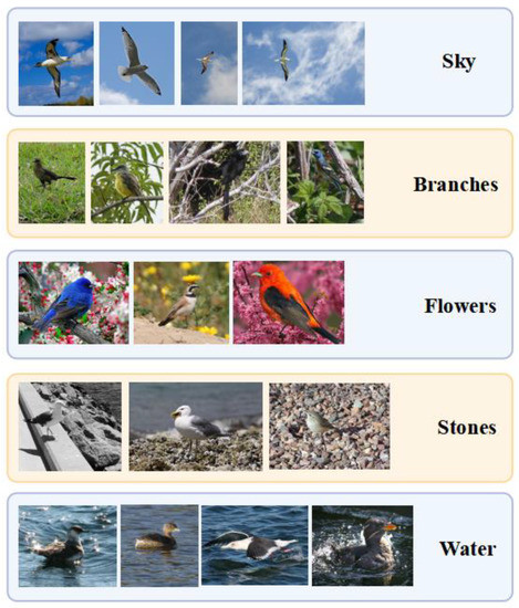
Figure 1. Complex backgrounds in CUB-200-2011.
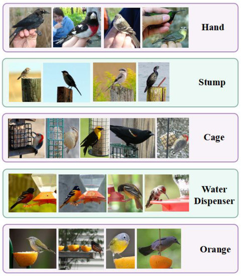
Figure 2. Variable pseudo-objects in CUB-200-2011.
Researchers present an MPDN for few-shot image classification that combines an instance-segmentation-based object localization (ISOL) module with a graph-based multilevel distribution propagation (GMDP) module to address these issues. The instance segmentation adopted by the ISOL module is based on prior knowledge. Using the previously known segmentation of the images, ISOL divides the raw images into segments based on the outer contour of the target object and masks the non-object portions. The final outputs of ISOL are the regions included in each object’s minimum bounding rectangle (MBR). The GMDP module, which consists of three graph networks concatenated in series, is used to post-process the features. The outcomes of GPDN are three layers of distributions with increasing abstraction. We then use these three distributions to update the original features that were supplied to the GMDP module, and we send the revised features back to the module to be used in the following iteration. Iterations serve the objective of making the final output features contain the information of the entire graph by repeatedly computing the distribution.
The steps for training the MDPN are as follows: Images are first supplied to the ISOL module. The ISOL module crops the images in accordance with the object’s MBR. After that, the cropped images are sent to the backbone to extract features. The GMDP module is then used to extract the three levels of distribution features from the object features, which are subsequently utilized to update the original object features. Following a number of iterations in the GMDP module, the cross-entropy loss between the output features of the GMDP module and the ground truth labels is determined.
2. Few-Shot Learning
Few-shot learning (FSL) can be broadly categorized into three ways: (1) using external memory; (2) introducing previous knowledge into the model initialization parameters; and (3) using training data as prior knowledge.
The first way to use external memory is to store training characteristics in an external memory and then compare test features with the features read from the external memory to predict the label of the test sample. Santoro et al. [5] first put forward the idea of using external memory to perform FSL problems in 2016, and their proposed memory-augmented neural network (MANN) can overcome the concerns with LSTM [6] instability. MetaNet [7], proposed by Munkhdalai et al., combines external memory and meta-learning. Qi Cai et al. [8] proposed a memory matching network that uses storage support features and the corresponding category labels to form “key-value pairs” in a memory module. Kaiser et al. [9] proposed a lifelong memory module that uses the k-nearest neighbor (KNN) to select k samples that are closest to the query sample and predicts the label of the sample. However, it should be noted that the extra storage space will increase the cost of training.
The second strategy, known as meta-learning, enables the model to learn how to learn by embedding prior knowledge into the model initialization parameters. MAML [10], a gradient-based method proposed by Finn et al. in 2017, designs a me-ta-learner as an optimizer to update model parameters with only a few optimization steps when given novel examples. The MAML-based Meta-SGD [11] algorithm can learn both the direction and the pace of optimization. Additionally, Nichol et al. [12] proposed Reptile in 2018, which greatly reduces the computational complexity by avoiding the computation of two derivatives in MAML. MetaOptNet [13] proposed replacing the nearest-neighbor method with a linear classifier that can be optimized for convex optimization learning.
The ways of using training data as prior knowledge are further divided into finetuning-based methods and metric-based methods. The goal of the former is to train the model using a lot of auxiliary data and then fine-tune it using the target few-shot dataset. The latter’s goal is to create a network that can distinguish between several classes by doing feature distance analysis. Many classical networks for few-shot classification are based on metric-based methods. MatchingNet [14] generates a weighted nearest neighbor classifier by computing the mapping distance between the support set and the query set. ProtoNet [15], proposed by Snell et al., extracts prototype features from samples of the same category and then predicts them by comparing the Euclidean distance between query features and prototype features. RelationNet [16] uses an adaptive nonlinear classifier to measure the relationship between support features and query features.
2. Attention Mechanism
The attention technique was initially employed in the machine translation problem and is now extensively used in several deep learning disciplines [4,17]. Humans selectively focus on a portion of all information while disregarding others due to the information processing bottleneck. Similar to how a human brain analyzes information, a neural network employs its attention mechanism to quickly focus on a small subset of important data.
Class activation mapping (CAM) [18] has recently gotten more and more attention. CAM works as follows: first, delete the convolutional neural network’s (CNN) last fully connected layers; Secondly, substituting a global average pooling (GAP) layer for the maxpooling layer; computing the characteristics’ weighted average comes last. However, it must change CNN’s structure, and accuracy must be gradually increased by training, which slows the model’s convergence rate. Then, a variety of enhanced CAMs have been put out to expand CAM to more intricate CNN structures: Grad-CAM [19] relies on gradients to weight features learned in the final convolutional layer and generalizes CAM without changing the model. Grad-CAM++ [20] improves Grad-CAM visualization by weighting the gradients pixel by pixel. CBAM [21] is a lightweight general-purpose module that can be smoothly integrated into any convolutional neural network architecture [22] to participate in end-to-end training. It infers the attention map along two distinct dimensions (channel and spatial).
Since the attention mechanism needs to be optimized over several iterations, it is time-consuming and not easy to locate and cover the entire object. The accuracy of the activation mechanism generally remains low because it often only focuses on a part of the object and may capture a lot of pointless information. We use instance segmentation methods in our object localization module to achieve accurate localization in order to prevent information redundancy and misinformation. The instance segmentation method approach accurately and completely obtains objects by masking off non-object regions to eliminate the interference of background and pseudo-objects. It makes feature extraction more effective.
3. Graph Neural Network
GNN has been heavily utilized in FSL recently. Garcia et al. [23] first suggested using GNN to solve few-shot image classification in 2018. They proposed to treat each sample as a node in the graph and use GNN to learn and update the embedding of the node, and then update the edge vector through the node vector. To further capitalize on intra-class similarities and inter-class differences, the conduction propagation network (TPN) [24] proposed by Liu et al. leverages the complete query set for inference.
Kim et al. [25] proposed an edge-labeled graph neural network, where the two dimensions of edge features correspond to the intra-class similarity and the inter-class difference of the two nodes connecting the edge, and then binary classification is performed to determine whether two nodes belong to the same class. Yang et al. [26] proposed the distribution propagation graph neural network (DPGN), which constructs an explicit class distribution relationship. Gidaris et al. [27] added denoising autoencoders (DAE) to GNN to correct the weights of few-shot categories. The GNN-based model is significant and should be explored widely because of its powerful information propagation and relationship expression abilities. Zhang et al. [28] proposed a graph information aggregation cross-domain few-shot learning (Gia-CFSL) framework, intending to mitigate the impact of domain shift on FSL through domain alignment based on graph information aggregation. Zhong et al. [29] presented a graph-complemented latent representation (GCLR) network for few-shot image classification to learn a better representation. A GNN is added to relational mining to better utilize the relationship between samples in each category.
This entry is adapted from the peer-reviewed paper 10.3390/app13116518
This entry is offline, you can click here to edit this entry!