Your browser does not fully support modern features. Please upgrade for a smoother experience.
Please note this is an old version of this entry, which may differ significantly from the current revision.
In the smart manufacturing sector, analyzing time series data is essential for monitoring plants and machinery to prevent costly failures or shutdowns. In order to gain new insights and make better control decisions, new methods are needed for extracting information and interpreting sensor data from hundreds of systems.
- aluminum electrolysis
- meta-features
- principal component analysis
- sensor data
- time series
1. Introduction
Due to advances in digitalization and the growing market in the smart manufacturing sector, most plants and machinery are now equipped with new sensor technology. The possible use cases of sensors can vary greatly: in the aluminum-production industry, sensors are used to monitor the state of reduction cells [1] or to measure individual anode currents [2] while in the food-refrigeration industry sensor data are analyzed to predict over-temperature disturbances [3]. To gain new insights about a system, the sensor data have to be preprocessed, analyzed and visualized in a compact way. However, manually analyzing the data from each sensor is a time consuming process. To tackle this problem new methods have to be developed that are capable of quickly extracting information and interpreting the sensor data from hundreds of systems.
Calculating certain features is a promising solution for quantifying the characteristics of a time series [4] which reduces the amount of data to a specific number of meta-features and can be understood as a dimensionality reduction technique [5]. According to [4], a representation of time series and similarity metric can be used in different fields, i.e., query by content, anomaly detection, motif discovery, clustering and classification. Furthermore, calculating meta-features is an essential part in the field of meta-learning to improve learning systems by incorporating already collected knowledge [6].
Meta-features should describe the “global picture” of a time series [5]. Specific time series meta-features, such as the trend (or trend-cycle) and seasonal strength, can be computed just like the mean or median. Examples of these meta-features can be seen in Figure 1, which shows different time series from the Makridakis Competitions, i.e., M1- and M3-Competition [7]. Strength values close to 1 indicate a strong trend or seasonal component in the corresponding time series. A strength value close to 0 indicates a weak trend or seasonal component in the corresponding time series.
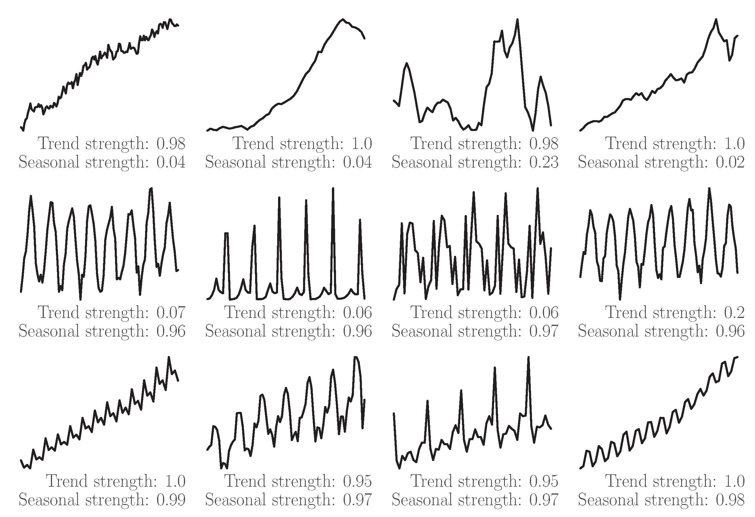
Figure 1. Several raw time series from the M1- and M3-Competition [7], which have different characteristics regarding the trend and seasonal strength. Values were rounded to two decimal places. Trend strength and seasonal strength were computed using feasts 0.1.6 [8]. Further examples can be found in [9].
Beside the trend and seasonal strength, more time series meta-features, e.g., the spectral entropy, seasonal period or autocorrelation coefficients, can be computed. Time series meta-features should be selected according to the type of the time series and the problem in question [9][10]. Expert knowledge about a specific domain, in the case the aluminum electrolysis, can help to find suitable meta-features that describe the different characteristics of time series.
The core business of TRIMET Aluminium SE is the development and production of aluminum products. Figure 2 shows one of the three pot rooms containing 120 reductions in an end-to-end configuration at the Essen site in Germany. In total, TRIMET Aluminium SE Essen (TAE) operates 360 reduction cells that produce liquid aluminum. The industrial production of aluminum is based on the Hall–Héroult process, in which alumina (Al2O3) is dissolved in liquid cryolite (Na3AlF6) with an excess of aluminum fluoride (AlF3) [11][12]. The Hall–Héroult process is performed with an almost constant energy supply to ensure stable aluminum production [12][13].
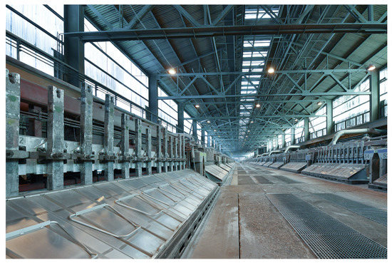
Figure 2. One of the three pot rooms operated at the Essen site in Germany by TRIMET Aluminium SE. One pot room contains 120 reduction cells in an end-to-end configuration (©TRIMET Aluminium SE).
Due to the energy transition, the energy supply in Germany is increasingly reliant on renewable energy sources, which means that the energy supply for the industrial aluminum production is no longer constant but variable [12]. In order to ensure a stable operation of the reduction cells with a variable energy supply, TAE has started to equip the reduction cells with magnetic field compensation and shell heat exchangers [14]. The magnetic field compensation is used to prevent bulging of the liquid aluminum at high current levels, while the shell heat exchangers are designed to control the heat loss from the side walls of the cells, maintaining a protective side ledge. Additional thermocouples are mounted on some cells to monitor the heat balance. Due to the corrosive environment, loose or faulty thermocouples are unavoidable and can result in incorrect heat balance calculations. Abnormal thermocouples are identified by manual evaluation of the recorded temperature signals (time series). However since hundreds of temperature signals have to be checked, this procedure is time consuming.
2. Literature Overview: Time Series Meta-Features
Grabowski et al. [15] calculated meta-features, i.e., the mean for numeric data and the sum for binary data, of several process variables in a rolling window to predict the bath temperature of reduction cells using a random forest. Kremser et al. [16] used several time series meta-features from [17][18] in a rolling window to predict anode effects in reduction cells using logistic regression, linear support vector machine, random forest and eXtreme Gradient Boosting.
Nanopoulos et al. [19] used a multilayer perceptron (MLP) and eight time series meta-features to classify patterns in control charts. The authors compared the performance of the MLP with another MLP that is solely based on the values of the time series. In further experiments, the performance of both MLPs was analyzed with noise corrupted time series and time series at varying length. Horvath et al. [20] used hierarchical clustering and seven parameters (meta-features) to divide reduction cells with similar behavior into control groups.
Hyndman et al. [21] computed 18 meta-features from time series representing the performance of servers at the internet company Yahoo. With the help of a principal component analysis (PCA), 𝛼-hulls and highest density regions, the authors used the calculated meta-features to identify entire time series that differed from other time series in the data set. In [22], the extreme value theory was used to identify anomalous streaming time series data. The presented framework is based on the calculation of 14 time series meta-features, which are used in an offline and an online phase. The offline phase is used to train a model on the typical behavior of the system. Afterward, the model was deployed in the online phase to identify anomalous time series using a rolling window. Furthermore, the authors present an algorithm that updates the model if a significant change in the distribution of the typical behavior of the system is detected. In a practical example, the authors used the framework to identify anomalous sensor data.
Kang et al. [23] computed six time series meta-features to visualize and analyze the M3-Competition data set [24]. The authors performed a PCA using the calculated meta-features, then visualized the first and second principal component (PC) to obtain an overview of the time series characteristics of the M3-Competition data set. Furthermore, the two-dimensional feature space and a genetic algorithm were used to generate new time series that extend the original data set. The authors then compared the feature space with the performance of selected forecasting methods. Talagala et al. present in [9] the FFORMS framework which includes the training of a classifier with time series meta-features to predict an algorithm that might be appropriate in forecasting a time series.
The authors in [25] applied the meta-learning approach to automate the process of selecting forecasting models for individual time series using meta-features. In their first case study decision trees with 10 meta-features calculated from stationary time series were trained to choose between two forecasting models. The second case study considers NOEMON [26] and five meta-features, which were calculated for each time series in the yearly M3-Competition data set [24], to rank forecasting models, i.e., random walk, Holt’s linear exponential smoothing, and auto-regressive model.
This entry is adapted from the peer-reviewed paper 10.3390/app13127065
References
- Majid, N.A.A.; Taylor, M.P.; Chen, J.J.J.; Stam, M.A.; Mulder, A.; Young, B.R. Aluminium process fault detection by Multiway Principal Component Analysis. Control Eng. Pract. 2011, 19, 367–379.
- Kremser, R.; Grabowski, N.; Düssel, R.; Kessel, K.; Tutsch, D. Investigation of Different Measurement Techniques for Individual Anode Currents in Hall-Héroult Cells. In Proceedings of the 12th Australasian Aluminium Smelting Technology Conference, Queenstown, New Zealand, 2–7 December 2018.
- Pursche, T.; Grabowski, N.; Nowitzki, J.; Claub, R.; Patryarcha, L.; Dreisbach, H.; Tibken, B. Identification of Overtemperature Disturbances in Industrial Food Refrigeration Processes. In Proceedings of the 2018 57th Annual Conference of the Society of Instrument and Control Engineers of Japan (SICE), Nara, Japan, 11–14 September 2018; IEEE: New York, NY, USA, 2018.
- Fulcher, B.D. Feature-Based Time-Series Analysis. In Feature Engineering for Machine Learning and Data Analytics; CRC Press/Taylor & Francis Group: Boca Raton, FL, USA, 2018; pp. 87–116.
- Wang, X.; Smith, K.; Hyndman, R. Characteristic-Based Clustering for Time Series Data. Data Min. Knowl. Discov. 2006, 13, 335–364.
- Vilalta, R.; Drissi, Y. A Perspective View and Survey of Meta-Learning. Artif. Intell. Rev. 2002, 18, 77–95.
- Hyndman, R. Mcomp: Data from the M-Competitions, R package Version 2.8. 2018. Available online: https://cran.r-project.org/package=Mcomp (accessed on 21 April 2023).
- O’Hara-Wild, M.; Hyndman, R.; Wang, E.; Feasts: Feature Extraction and Statistics for Time Series. R package Version 0.1.6 (conda-forge). 2020. Available online: https://cran.r-project.org/package=feasts (accessed on 21 April 2023).
- Talagala, T.S.; Hyndman, R.J.; Athanasopoulos, G. Meta-learning how to forecast time series. J. Forecast. 2023.
- Kang, Y.; Hyndman, R.J.; Li, F. GRATIS: GeneRAting TIme Series with diverse and controllable characteristics. Stat. Anal. Data Mining ASA Data Sci. J. 2020, 13, 354–376.
- Grjotheim, K.; Kvande, H. Introduction to Aluminium Electrolysis: Understanding the Hall-Héroult Process, 2nd ed.; Alu Media GmbH: Düsseldorf, Germany, 1993.
- Düssel, R. Entwicklung eines Regelungskonzepts für Aluminium-Elektrolysezellen unter Berücksichtigung einer Variablen Stromstärke und eines Regelbaren Wärmeverlusts. Ph.D. Thesis, Bergische Universität Wuppertal, Wuppertal, Germany, 2016.
- Depree, N.; Düssel, R.; Patel, P.; Reek, T. The ‘Virtual Battery’—Operating an Aluminium Smelter with Flexible Energy Input. In Light Metals 2016; Springer: Cham, Switzerland, 2016; pp. 571–576.
- Düssel, R.; Mulder, A.; Bugnion, L. Transformation of a Potline from Conventional to a Full Flexible Production Unit. In Light Metals 2019; Chesonis, C., Ed.; Springer: Cham, Switzerland, 2019; pp. 533–541.
- Grabowski, N.; Kremser, R.; Düssel, R.; Mulder, A.; Tutsch, D. Using Random Forest Regression for Predicting and Analysing Reduction Cell Behaviour. In Proceedings of the 12th Australasian Aluminium Smelting Technology Conference, Queenstown, New Zealand, 2–7 December 2018.
- Kremser, R.; Grabowski, N.; Düssel, R.; Mulder, A.; Tutsch, D. Anode Effect Prediction in Hall-Héroult Cells Using Time Series Characteristics. Appl. Sci. 2020, 10, 9050.
- Lubba, C.H.; Sethi, S.S.; Knaute, P.; Schultz, S.R.; Fulcher, B.D.; Jones, N.S. catch22: CAnonical Time-series CHaracteristics. Data Min. Knowl. Discov. 2019, 33, 1821–1852.
- Garza, F.; Gutierrez, K.; Challu, C.; Moralez, J.; Olivares, R.; Mergenthaler, M. tsfeatures. Python Package. Available online: https://github.com/Nixtla/tsfeatures (accessed on 21 April 2023).
- Nanopoulos, A.; Alcock, R.; Manolopoulos, Y. Feature-Based Classification of Time-Series Data. In Information Processing and Technology; Nova Science Publishers, Inc.: Hauppauge, NY, USA, 2001; pp. 49–61.
- Horvath, M.; Vircikova, E. Data Mining For Quality Control of Primary Aluminium Production Process. In Management and Production Engineering Review; Production Engineering Committee of the Polish Academy of Sciences, Polish Association for Production Management: Warsaw, Poland, 2012; Volume 3, pp. 47–53.
- Hyndman, R.J.; Wang, E.; Laptev, N. Large-Scale Unusual Time Series Detection. In Proceedings of the 2015 IEEE International Conference on Data Mining Workshop (ICDMW), Atlantic, NJ, USA, 14–17 November 2015; IEEE: New York, NY, USA, 2015.
- Talagala, P.D.; Hyndman, R.J.; Smith-Miles, K.; Kandanaarachchi, S.; Muñoz, M.A. Anomaly Detection in Streaming Nonstationary Temporal Data. J. Comput. Graph. Stat. 2020, 29, 13–27.
- Kang, Y.; Hyndman, R.J.; Smith-Miles, K. Visualising forecasting algorithm performance using time series instance spaces. Int. J. Forecast. 2017, 33, 345–358.
- Makridakis, S.; Hibon, M. The M3-Competition: Results, conclusions and implications. Int. J. Forecast. 2000, 16, 451–476.
- Prudêncio, R.B.C.; Ludermir, T.B. Meta-learning approaches to selecting time series models. Neurocomputing 2004, 61, 121–137.
- Kalousis, A.; Theoharis, T. NOEMON: Design, implementation and performance results of an intelligent assistant for classifier selection. Intell. Data Anal. 1999, 3, 319–337.
This entry is offline, you can click here to edit this entry!