Your browser does not fully support modern features. Please upgrade for a smoother experience.
Please note this is an old version of this entry, which may differ significantly from the current revision.
Subjects:
Engineering, Civil
With the increasing capabilities of computational systems, reliable algorithms can be applied to a wide variety of case studies, including those found within the wave energy sector. Some of the most advanced tools are supported by Big Data and employ artificial intelligence (AI) towards estimating local wave energy resource, forecasting operational or extreme wave conditions, or filling data-gaps in wave field measurements.
- renewable wave energy
- artificial intelligence
- metaheuristic algorithms
- wave energy resource
- wave climate forecasting
- neural networks
1. Introduction
Improving energy conversion technologies has been a key objective towards ensuring a reliable and sustainable energy supply to human activities. After decades of investment in fossil-fuel-based systems, investors and researchers set their sights on renewable energy sources (RES)—mainly wind, solar and hydropower—to promote a greater energy mix and an energy transition towards more environmentally friendly solutions. This promoted long-term research, learning curves and investments, which resulted in increasingly lower costs of RES [1] at greater scales, deployed capacity, reliability and efficiency [2]. RES have become economically competitive with fossil fuels, but the latter still retain a global supply market share of about 80.9% [3]. Thus, further efforts must be put into developing and deploying RES.
At sea, the scenario is different. Aside from the growing energy production injected into mainland electrical grids, the advent of promising markets, from aquaculture [4] to desalination [5], as well as the necessity of green transition within seaports [6] have prompted a significant penetration of RES, particularly solar [7] and offshore wind [8]. They also enable a greater degree of autonomy at sea for floating systems, such as buoys. Even so, there may be more suitable energy alternatives within the ocean environment. In particular, wave energy has received significant attention, given its high energy density, forecasting accuracy and availability [9,10]. Currently, hundreds of different concepts are being developed, but this has not ensured a design convergence or a sufficient degree of maturity for the wave energy sector to be commercially competitive [11,12]. One of the major issues derives from the optimization problem of wave energy converters (WECs). Several variables are required for a suitable development, from structural design to Power Take-Off (PTO) configuration, to which adds nonlinear wave–structure interactions. Standard practices towards improving the WECs include physical [13] and numerical modelling [14] campaigns. Depending on their goals and methods, they can be demanding in both time (days to weeks), effort (learning curves and data processing) and logistics (model configuration, construction and setup), whilst not ensuring a sufficiently optimized solution towards commercial viability. Complementary algorithmic tools can enable a more thorough and automated sweep of alternative design solutions, at much lower computational effort and time. In fact, this has already been demonstrated for other energy technologies, as highlighted in [15,16].
With the increasing capabilities of computational systems, reliable algorithms can be applied to a wide variety of case studies, including those found within the wave energy sector. Some of the most advanced tools are supported by Big Data and employ artificial intelligence (AI) [17]. In this regard, a summarized taxonomy can be found in [18], which also features a review of WEC park layout optimization supported by AI techniques. An extended classification is provided in Figure 1, adapted to the main algorithms discussed in this research. A distinction is made between “indirect” and “direct” optimization algorithms. While the former are more oriented towards wave propagation, body motion prediction and/or gap filling (e.g., required for resource matrices and time series completion) [19], the latter tend to more directly solve optimization problems, from WEC design to parameter minimization/maximization. Indirect algorithms are, furthermore, designated upon a necessity of data interpolation for pattern identification, based on regression and classification approaches. Specific examples can be found in Artificial Neural Networks (ANNs), Support Vector Machines (SVM) and Random Forests (RF). The direct algorithms are considered when an optimization problem within a set search space exists, aiming at minimizing/maximizing a concrete objective function [20]. Ideally, the global optimal solution can be found over existing local minima/maxima, thus avoiding the vanishing gradient problem found in other techniques (e.g., ANNs [21]). The most common algorithms are (or operate with) metaheuristic and attempt to mimic certain natural patterns, such as evolution—Evolutionary Algorithms (EA)—population and individual behaviour—Swarm Intelligence (SI)—and nonbinary bounded human logic—Fuzzy Logic (FL). Complementary tools such as Principal Components Analysis (PCA), Model Predictive Control, Harmony Search Algorithm, Covariance Matrix Adaptation Evolution Strategy and regression techniques can also be considered.
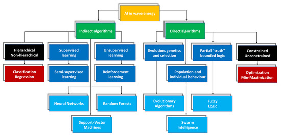
Figure 1. Categorization of the most commonly applied “direct” and “indirect” AI-based optimization algorithms.
The potential applications of such algorithms to wave energy development are immense, and not limited to electricity generation:
-
A recent study by Mares-Nasarre et al. [22] resorted to an explicit ANN-derived formula for estimating overtopping layer thickness and overtopping flow velocity on rubble-mound breakwaters, subjected to depth-limited wave breaking conditions. A total of 235 2D experimental tests were performed to obtain data for developing the ANN-based formulae, from which it was found that the Iribarren number and dimensionless crest freeboard were the key variables;
-
Schmitt et al. [23] configured a numerical wave tank within OpenFOAM through the application of ANNs, mainly to approximately “solve” the Navier-Stokes equations and obtain nonlinear tank transfer functions required for the wavemaker. In total, 800 out of 1000 samples of wavemaker input were applied to train the ANN (80-20 training-validation ratio), during which a mean square error (MSE) was used as the loss function. The ANN was composed of two hidden layers with 310 nodes, to which were added the input and output layers. The hyperbolic tangent (tanh) and linear activation functions (AFs) were used for 350 training epochs. Details on the software (Python) and hardware can be found in [23]. As a result, a fast and reliable prediction of the desired waves, which were measured via a numerical wave gauge, was obtained;
-
Guo et al. [24,25] employed a long short-term memory (LSTM)-based machine learning model, a type of recurrent neural network (RNN), to predict future surge and heave motions of a semi-submersible. A step-decay algorithm was used for the learning rate schedule, set at 0.01 for the first 10 epochs, followed by a decayed rate of 0.1 for every 50 epochs (200 maximum). Two LSTM layers with 200 output layer neurons were configured, which incorporated five fully connected blocks of 80 neurons each. The tanh was the AF, while the Adaptive Moment Estimation (Adam) optimizer was selected. A high degree of correspondence was obtained (~90%), and it was found that, for any single point prediction, the outputs from the LSTM model followed a Gaussian distribution;
-
Sirigu et al. [26] resorted to a genetic algorithm (GA) combined with a boundary element method code to perform a holistic optimization of the PeWEC device [27]. Several bounded study variables were considered for optimization, including the hull (6), the PTO (2) and the pendulum component (5). As objectives, three fitness functions were defined—minimize capital expenditures over productivity, maximize the capture width ratio (CWR) and mitigate manufacturing/weight costs—resulting in a multi-objective Pareto optimal set. GA convergence was achieved after less than 120 generations. The results point to significant, yet diverging gains, in the sense that beneficial design alterations that increase the CWR, for instance, may cause a detrimental cost increment (to which minimization priority is given);
-
A more concrete application can be found in the recently established partnership between EMEC and H2GO Power, HyAI [28], where offshore renewables (including wave energy) are deployed towards electricity generation for hydrogen production. To optimize the operations, an AI software-controlled hydrogen storage technology is employed for data-driven asset management decisions in real time.
2. Algorithm Overview
2.1. Indirect Algorithms
2.1.1. Neural Networks
The underlying principle behind ANNs is the human brain, namely the neurons and their components, Figure 2. Mimicking, to some extent, the way that information is transmitted from one neuron to the next, ANNs can identify patterns, classify, approximate and interpolate outputs (output layer) based on a set of input data (input layer), so long as it is adequately “trained” (e.g., avoids overfitting). The fundamental architecture incorporates, aside from the input and output layers, one or more “hidden” intermediate layers where the information is processed—a black-box model. The input data, or “nodes”, are passed through one layer made up of “neurons”. For one of the most common subtypes of neural networks, ANNs, two hyperparameters must be defined for each neuron—a weight and a bias—either randomly or via an optimization technique. A net input is obtained after the original input data are multiplied by the neuron’s weight and modified by its bias. This net input is then passed through an AF [29]—rectified linear unit (ReLU), tanh, sigmoid and Softmax, among others—which defines whether the neuron is active or not, and to what degree. Depending on the network architecture, the resulting data are carried directly to the output layer (single hidden layer) or indirectly, first passing through the neurons of another hidden layer and serving as input data for them (multilayer) [30].
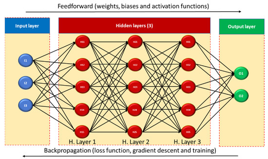
Figure 2. Schematic of the basic architecture for an Artificial Neural Network (fully connected, supervised deep network).
In some cases, the neurons of one hidden layer can be fully connected to neurons from another layer and incorporate nonlinear AFs. This is designated as the Multilayer Perceptron (MLP), which enables identification of nonlinear patterns between input and output data. Moreover, the MLP is a class of ANNs [31] which requires two key operating processes—feedforward and backpropagation. The former has been summarized in the previous paragraph, while the latter implies the calculation of a loss function. This step is required to check the quality of the obtained results versus the expected ones. Should the difference surpass a specified limit, an iterative process occurs in which the loss is backpropagated through the hidden layers to update the hyperparameters with more suitable values. The adjustment can be improved through gradient descent algorithms, although control of vanishing gradient should be exercised. The iterative process of feedforward and backpropagation occurs over numerous iterations until the stopping condition is met (e.g., loss below a certain threshold). This process is first employed for training purposes, in which a portion of the input data (e.g., 80%) is used to train the ANN towards finding the desired outputs, while the remaining portion is used for validating it. The training can be tracked through its learning rate and loss function evolution over the iterations/epochs. The learning processes are commonly either supervised (input and output are given), unsupervised (self-organize to reach the output), semi-supervised (partially labelled data) or reinforced (learning based on reward mechanism).
Another subtype of neural networks is the convolutional neural networks (CNNs) [32], in which the weight matrices are created from convolution with filter masks, mainly for pattern recognition across space. The CNNs’ hidden layers are, in fact, convolutional layers where the input is taken and convolved, for each neuron, over a matrix filter to produce the corresponding output, which is then passed on to the next layer. As such, it is pivotal to define the number of filters and the values found within the inherent matrix. In the field of wave energy, there is equal interest in finding patterns across time, such as wave climate hindcasting and forecasting. A suitable tool can be found in the form of RNNs [33], in which the connection scheme enables a “memory” effect: the input of a hidden layer derives from the preceding layer’s output and its own output from the previous time-step. This internal information flow—input, weight and output vectors—creates a loop between subsequent time-steps and is designated as “hidden state”, which is also regulated by AFs. Therefore, they represent the outputs of the hidden layers and are subject to update for each time-step, depending on the previous time-step’s hidden state and the current input. This summarizes the standard principles of RNNs, but modified variants exist, namely to counter the vanishing gradient problem and consequent short-term memory issues. Among them are the LSTM [34] and gated recurrent units (GRUs) [35], which apply forget/input/output gates alongside a cell state and update/reset gates with a hidden state, respectively, to regulate the flow of information. In other words, these mechanisms control which information should be stored—and passed on to the following step or state—or forgotten.
2.1.2. Random Forests
A different indirect method applied in the wave energy field of research is related to ensembles of decision trees. Although standard decision trees permit an intuitive, straightforward and fast classification process, they are prone to accuracy and generalization issues for variable datasets, thus demonstrating relatively low adaptability. Complexity can also cause overfitting of the data. To circumvent these problems, the RF approach is applied, where a multitude of random decision trees is employed [36,37], Figure 3. In essence, each decision tree is randomly constructed in a subspace of the feature space using the entire training dataset. For training purposes, the process of bootstrapping aggregating, or bagging, is used, in which training subsets are initially randomly sampled from the original dataset, with replacement. A “forest” is generated from the different trees originated out of each subset, which can be used for validation purposes—bootstrapping. For instance, validation data can be passed through this ensemble of decision trees, resulting in different predictions that can be combined—aggregation. A final selection of the most adequate outcome is performed through a discriminant function, which can operate through prediction averaging (regression) or “majority vote” (classification), depending on the nature of the case study. Consequently, the trained model is less sensitive to variance in the original dataset whilst retaining significant accuracy, as different datasets are applied for each tree and the correlation between different trees is controlled, ensuring greater solution diversity. Even so, this comes at the expense of harder interpretation, as the bagging process is more intricate than the standalone decision tree configuration. Lastly, a recent study addresses the convergence rate of different random forest variants, for a classification problem [38], from which similar RF convergence rates were obtained for multi-class learning and binary classification, albeit with alternative constants.
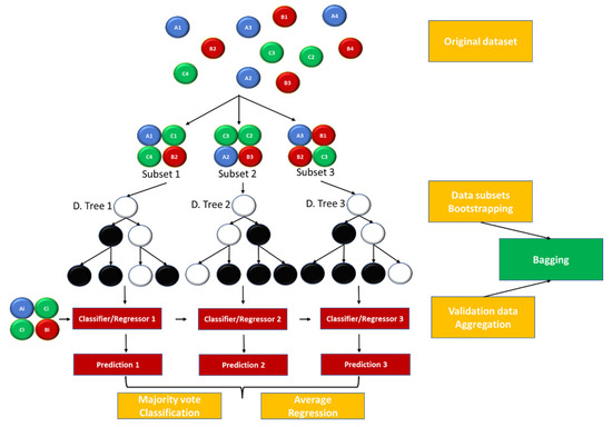
Figure 3. Simplified schematic of the underlying principles behind the Random Forests algorithm (supervised, non-hierarchical example).
2.1.3. Support Vector Machines
Although additional techniques exist, a third indirect algorithm that is commonly applied in studies on wave conditions will be addressed, here, to close this subsection: the SVM approach. Following on the schematic in Figure 4, one starts with an nth dimensional dataset that can be either categorized, regressed or swept for outliers. Assuming the former as an example, it is pivotal to ensure that an adequate classification is obtained, which promotes generalization for new datasets and their accurate labelling [39]. As such, one must accurately define a separation threshold between the different data types. This also implies setting a margin between reference points from each data type. In linear problems, such a margin can fully restrict potential classification errors from data outliers—hard margin—or enable some degree of error—soft margin. The former does not allow for training errors but can be very sensitive to outliers of one data type in the vicinity of another data type, while the opposite is found for the latter. Soft margin also demonstrates higher generalization and can be adjusted through slack variables ξ. In fact, a hard margin can be perceived as a soft margin with such variables set to 0. To control the complexity–training accuracy trade-off and mitigate overfitting risks, a penalty factor is also employed. These steps enable the definition of n − 1th dimension support vector classifiers, or hyperplanes, separating the data types. An optimal hyperplane ought to maximize the margin, and in SVM it can be found at a higher data dimension by kernel functions, including for nonlinear problems. In reality, the relationships between the data types does not require an actual transformation of said data into higher dimensions, but rather a projection of them onto which the kernels perform the relationship assessments, at said higher dimensions—kernel trick—thus avoiding the need for computing the data transformations. Different kernels can be selected, but the most commonly employed and nonlinear are the polynomial, the Gaussian radial basis function and the tanh/sigmoid [40].
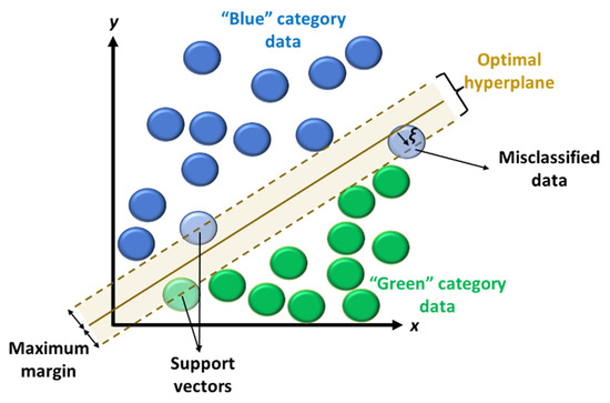
Figure 4. Two-dimensional data space with a soft-margin linear application example of Support Vector Machines (supervised, non-hierarchical example).
SVMs have demonstrated superb capabilities with regard to generalization and classification error mitigation (reliable results upon cross-validation). However, large datasets can lead to significant computational requirements, while multiple binary classification problems present a very complex challenge that is commonly addressed through one-against-all or one-against-rest approaches. Furthermore, imbalanced datasets can lead to suboptimal separation hyperplanes, causing lower accuracy and high bias towards minority classes. Some solutions have been proposed, including a combined application with “direct” algorithms, such as GAs [41] and FL [42], to balance out the datasets and optimize the SVM parameters. In fact, these and other “direct” algorithms are the subject of the next subsection of this research. An in-depth assessment of SVM fundamentals, implementations, advantages and disadvantages can be found in [40].
2.2. Direct Algorithms
2.2.1. Evolutionary Algorithms
As a follow-up to the previous subsection, the direct algorithms are hereafter described. The underlying premises tend to mimic a certain natural phenomenon, depending on the selected technique. The first to be discussed are based on evolution and natural selection—Evolutionary Algorithms. Distinct techniques exist, such as Genetic Programming, Evolutionary Programming, Evolution Strategies, Differential Evolution and Genetic Algorithms [18]. However, the key premises remain [43]:
-
Generate an initial population of individuals/candidate solutions found within the search space;
-
Iteratively perform three tasks—evaluate an objective/fitness function for each individual, select the most “fit” individuals and apply variation operators to them in order to create a new generation of individuals towards an optimal solution;
-
Execute the iterative process over various generations until the stopping criterion is met.
One of the most commonly applied EA tools are Genetic Algorithms [44]. GAs start with an initial population of individuals (usually random) which is modified over the course of several generations to promote the existence of “fitter” individuals, capable of providing a suitable solution for the optimization problem. Each individual has a set of parameters, or “genes”, that categorize it as a potential problem solution. Even so, it is pertinent to promote an adequate level of population diversity for a better application of the GA algorithm (accuracy versus convergence). The selection or exclusion of individuals is performed by their scores with regard to a fitness function, which is specified by the user. This function can be discontinuous, stochastic, (un)bounded, non-differentiable or nonlinear. For the creation of a new generation, three main tasks are required:
-
Selection—as mentioned previously, the individuals with the best fitness function scores, or “parents”, are selected for producing the next generation, or “children”. To that end, fitness scaling can be applied, initially, so that an adequate comparison can be established. As a follow-up, a selection function is used to determine which individuals will be the parents of the next generation. Distinct rules can be applied, such as stochastic uniform, remainder, roulette or tournament. This is usually conducted with a ranking system (highest sorted fitness scores), but a top system (a fixed number of selected individuals with equally set scores) can be employed as an alternative. It is worth noting that the top system, albeit more straightforward in selecting fit individuals, promotes less diversity than the ranking system;
-
Reproduction—the selected parent individuals are conjugated to “reproduce” children of the next generation, analogous to the biological reproduction process found in nature. Even so, it may be of interest to keep some of the parents with the best fitness scores for the following generation, or “elite children”. They should be carefully defined, though, as an excessive amount may lead to unwanted dominance over the remaining population, thus reducing the algorithm’s effectiveness. To that end, a crossover fraction is established, whose value defines the percentage of newly created individuals, aside from the elite children, and depends on the case study characteristics. Reference fractions will be provided along this research;
-
Mutation and crossover—two key processes associated with reproduction, mutation and crossover promote the creation of non-elite children solutions distinguishable from their parents. Crossover children result from direct “reproduction” between two parents, where the respective “genes” are combined into a new configuration (e.g., a new vector entry of parameters). Numerous options exist for performing crossover, such as single-point or two-point swapping of vector entries at a given index(es), or even by applying a heuristic or scattered approach, among others. As for mutation, it is a process that also mimics the natural mutations that occur in genes. In GAs, mutation is applied to one individual in each pair of parents. A random change in the parent’s “genes” occurs (e.g., randomly changing a value in the vector entry of parameters). The mutation can be controlled through an uniform, Gaussian or adaptable function, among others, and is transmitted to the children. While mutation promotes diversity within the population, prompting the existence of potentially “fitter” individuals, crossover ensures the transmission and recombination of the best “genes” from the parent generation to the children generation.
The aforementioned tasks are repeated for each generation until a termination criterion is met, thus providing an optimized solution to the studied problem. While EAs provide a varied set of techniques to handle numerous optimization problems, which are constantly being upgraded, they are not without problems. A straightforward issue falls on the selection of not only the technique, but also the adequate hyperparameters and settings (e.g., selection, reproduction and mutation rules). Premature convergence towards suboptimal solutions can also occur, and finding an optimal trade-off between exploitation and exploration properties is equally challenging [46]. Even so, they have demonstrated their capabilities when handling WEC-related problems, such as parameter optimization (shape and damping) [47,48] or wave farm layout [49,50]. They can be equally applied to problems related with wave climate and resource, as addressed in this research.
2.2.2. Swarm Intelligence
Whereas EAs focus on reproducing the biological processes of evolution, gene transmission and natural selection, SI algorithms attempt to mimic the collective behaviour of a self-organized population. In detail, the original proposition revolves around artificial life systems—boids—which are defined by a position and velocity vectors and can simulate flocking behaviour [51]. By applying a set of rules to these simplistic artificial lifeforms—separation (direct contact/collision avoidance), alignment (movement towards the average direction of local units) and cohesion (movement towards the centre of gravity of local units)—higher-level complex behaviours emerge, which can be tuned to solve optimization problems. Once again, distinct metaheuristic algorithms exist, such as Ant Colonies, Artificial Bee Colonies, Glowworm Swarming or Particle Swarm Optimization (PSO), among others [18]. Within the wave energy field of research, the latter is more commonly applied to solve optimization problems. PSO was originally conceived in the late 1990s [52,53], but it has seen significant application and improvement since then [54]. In terms of implementation and algorithm convergence, the following steps are required, Figure 6:
-
Initialize a random set of swarm particles within the search space, each with an inherent initial position x0 and velocity v0 vectors;
-
Define and compute a fitness function to evaluate each particle, at its current position. This initial evaluation is to be repeated iteratively afterwards, as each particle’s new position should be assessed and compared, in terms of fitness, with its best previous position. Therefore, the best position is updated only if the current position yields a better fitness than the previous best;
-
At each time-step t, update the position xt and velocity vt vectors of each particle. Its new position results from the previous position xt−1 adjusted by a new velocity vector. Aside from the previous velocity vt−1—inertial term—this vector considers the particle’s best fitness history Pb (and inherent position and velocity)—cognitive/personal term—as well as the best fitness/position/velocity found within the swarm gb—social term. It is worth noting that each of these three terms is weighted by a hyperparameter, and tuning them presents a pivotal challenge in each case study;
-
Evaluate the best global fitness from the personal best of each particle in the swarm. This should be executed in conjunction with the previous step, so that the particles’ new positions can be updated. The global best should then be assessed through a termination criterion: should the result meet the termination target, then the algorithm stops, and the best solution is provided. Otherwise, the algorithm carries on with the previous steps, iteratively, until the termination criterion is met.
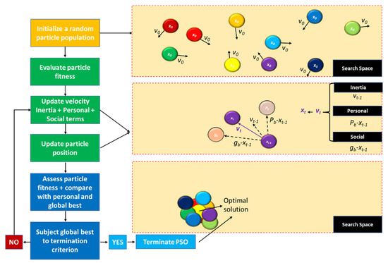
Figure 6. Schematic of the optimization process and steps in the Particle Swarm Optimization algorithm.
Although relatively simple to configure and execute, PSO can exhibit some application difficulties, such as setting up the swarm size or defining the number of iterations required towards convergence, as they affect the model’s accuracy and computational effort. It can be equally challenging to define an adequate set of hyperparameters, although reference values exist. Recommendations on parameter tuning for both evolutionary and swarm-based algorithms, including PSO, can be found in [55].
2.2.3. Fuzzy Logic
FL [56] addresses problems where the logical reasoning is nonbinary, Figure 7. In other words, it is not necessarily a “true” or “false” statement definition (e.g., integer value of 1 or 0), but rather a degree of truth that ranges in between (e.g., between 0 and 1)—partial truth. This follows on human interpretation, where the concept of vagueness overrules classical logic. From a practical perspective, FL takes in the input variables from a case study and, in general, executes the following tasks [57,58]:
-
Fuzzification—the input data, also designated as “crisp” inputs, are introduced into the algorithm and subjected to a fuzzification procedure that converts it into fuzzy datasets/variables. This is achieved through implementing membership functions, from which a membership degree can be attributed to the input. Such a degree is usually bounded by an upper and lower limit (e.g., 0 and 1), but it can be any value in between (e.g., 0 < degree < 1) and represents the degree of partial truth inherent to FL. The degree of a given input is a combination of each membership value that intercepts, vertically, one or more user-defined membership functions, which can be triangular, gaussian, trapezoidal or sigmoid in shape, among others;
-
Fuzzy inference with operators—following on the fuzzification process, the fuzzy variables are passed through a set of user-defined rules (e.g., IF-THEN) controlled by logical operators. The original Boolean operators, such as AND, OR and NOT, are substituted with corresponding fuzzy operators: Min(input), Max(input) and 1-Input (note that the input, here, is the fuzzy variables). This allows for the output fuzzy variables to be inferred from the input fuzzy variables, as the former are required for the next step;
-
Defuzzification—the inferred fuzzy variables are used, here, to obtain the final output crisp values. Each fuzzy variable is introduced into a new set of user-defined membership functions—trapezoidal, triangular or other shapes. There are numerous methods to apply defuzzification, such as Bisector, Smallest/Middle/Largest of Maximum or Centroid, although the latter is more commonly used. They “fill up” each membership function, based on the degree of membership to each, and one of the defuzzification methods is applied to acquire the final crisp values.
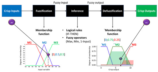
Figure 7. Schematic on the application of the Fuzzy Logic algorithm.
In the wave energy field of research, FL can be employed, for instance, towards configuring control systems for optimal WEC operation [59]. However, it can also be used towards predicting wave parameters [60], of greater interest to the scope of this research, or WEC design and deployment decision-making [61], as well as being employed alongside metaheuristic-driven optimization algorithms [62]. As such, although regarded, in this research, as a “direct algorithm”, it can be applied in indirect optimization problems.
3. Applications of AI-Based Algorithms to Wave Energy Studies
3.1. Introduction
The following subsections summarize reference applications of AI-based algorithms to case studies in which wave propagation modelling and assessment of wave conditions were required. Complementarily, Cuadra et al. [17] conducted an extensive study about AI for wave energy, including some topics discussed here. In detail, the present research focused on post-2016 research, which, based on previous knowledge and searches by keywords in journal repositories with a snowballing technique, comprises more than 60 different papers. Although most of the studies resorted to indirect algorithms (mainly ANNs, Figure 8), as defined previously, several cases in which direct algorithms are employed will also be presented and discussed, as well as complementary modelling techniques.
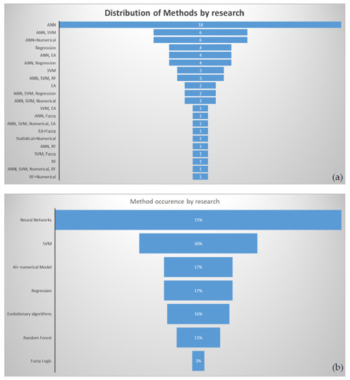
Figure 8. Distribution, in the literature, of AI-based algorithms applied to wave energy conversion (period of 2016 to 2022), by: (a) number of methods and (b) occurrence frequency.
3.2. Neural Networks Applied to Wave Propagation, Prediction and Energy Resource Estimation
As seen previously, one of the most often employed group of algorithms is neural networks, particularly ANNs. Even so, in several studies, more than one AI algorithm was applied, but the following subsections partition will conserve the distribution patterns found in Figure 8. Furthermore, many studies address topics related to estimating the available wave energy resource, as well as forecasting and gap-filling data related to wave climates, under operational conditions. This is pivotal towards WEC design optimization, in order to promote resonance occurrence, as well as estimating energy cost (e.g., Levelized Cost of Energy) and efficiency (e.g., Capacity Factor and CWR) metrics [63]. This subject is the core of the present subsection.
Looking at specific studies, Abhigna et al. [64] analysed the prediction of significant wave height (𝐻𝑠) using various ANN algorithms. The data were collected from a moored buoy in the Bay of Bengal for a two-year period, with the first year used for training and the second year used for prediction. According to the findings, the RNN that used the Bayesian Regularization algorithm demonstrated superior performance, as evidenced by a high correlation coefficient and a low MSE. However, the overall performance of the neural network still needs to be improved for more accurate predictions. Berbić et al. [65] applied ANN and SVM for forecasting 𝐻𝑠 in near real time for two locations in Australia. The algorithms’ forecasting ability was tested for different time periods, ranging from 0.5 to 5.5 h. The study found that using a smaller number of input attributes (e.g., three or six 𝐻𝑠 values) resulted in forecasts that are more accurate. They suggest that both ANNs and SVMs can be useful, with ANNs being suitable for shorter forecasting periods and SVMs for longer periods.
Mahmoodi et al. [66] used three different data mining methods (FFNN, CFNN and GEP) to estimate wave energy flux using meteorological data (wind speed, air and sea temperature) as input. The accuracy of the methods was evaluated using performance evaluation criteria (root mean square error (RMSE) and regression coefficient), and it was found that the FFNN method was the best in terms of accuracy. The study also found that there is a good correlation between wave energy flux and meteorological parameters, and that it is possible to estimate wave energy flux in areas without wave records. In a second study, Mahmoodi et al. [67] used machine learning methods, such as nonlinear autoregressive (AR) NNs, group method of data handling (GMDH) networks and LSTM networks, for forecasting the wave excitation force, which is the force exerted on a two-body heaving point absorber due to wave motion, for this study. The authors compare the performances using mean absolute error (MAE), RMSE, correlation coefficient and scatter index. They found that the nonlinear AR-NN generally provided the most accurate and reliable results for short-term wave elevation and wave excitation force forecasting, whereas the GMDH network performed well for longer time horizons. The LSTM network, on the other hand, gave mixed results depending on the dataset.
Guijo-Rubio et al. [68] analysed the performance of four different types of multi-task evolutionary artificial neural networks (MTEANNs) in predicting marine energy flux. The input data were from three buoys in the Gulf of Alaska and seven variables from reanalysis data. The MTEANNs were tested at different time prediction horizons (6 h, 12 h, 24 h and 48 h). The combination of sigmoidal units in the hidden layer with linear units in the output layer was found to perform best among the four MTEANN models tested and more traditional approaches, such as Support Vector Regression (SVR) and Extreme Learning Machine (ELM). Gómez-Orellana et al. [21] used the MTEANN to simultaneously predict short-term 𝐻𝑠 and wave energy flux in two different coastal zones in the United States: the Gulf of Alaska and the southwest coast of the United States. The model was trained with data from three buoys in each zone and compared against standalone MTEANN models trained for each buoy and against other popular regression techniques. The results showed that the MTEANN model using a zonal strategy (MTEANNZ) had the best performance in terms of MAE and standard error of prediction, whereas other linear models had lower complexity. The authors also found that the MTEANNZ model was able to capture the nonlinear behaviour of the wave data and had good generalization capabilities.
Sadeghifar et al. [69] used RNNs called nonlinear AR exogenous inputs to predict wave height H at various time intervals. The use of RNNs with different training functions showed improvement in the prediction of wave height, with a high correlation coefficient of 0.96 for 3-h predictions and 0.87 for 12-h predictions. The model was found to be more accurate in predicting higher waves and was demonstrated to be useful in various coastal engineering and oceanography applications. Kumar et al. [70,71] presented machine learning approaches for predicting daily H at various locations around the world. In [71], the Minimal Resource Allocation Network and Growing and Pruning Radial Basis Function algorithms were found to outperform ELM and SVR in predicting daily wave heights at 13 stations in the Gulf of Mexico, Korean region and UK region, requiring relatively few network resources. In [70], the authors presented the ELM Ensemble approach, which involves using multiple ELMs with different input parameter initializations. It was found to outperform other machine learning approaches such as SVR, ELM and Ordered Subsets ELM in predicting daily H. The approach was tested on wave data and atmospheric conditions from 10 stations in the Gulf of Mexico, Brazil and Korean region.
Wang et al. [72] presented a model based on deep neural networks, or DNNs, to calculate the mean wave period T from altimeter observations and signal parameters. The model is trained using data from the National Data Buoy Center (NDBC) buoys and observations from the Jason-3 satellite. The model included 𝐻𝑠, 𝐻𝑠 standard deviation and the 𝐻𝑠 gradient as input variables to account for the dependency of the wave period on these parameters. The DNN model was found to provide accurate results with a RMSE of 0.57 s and a scatter index of 9.7%. The model was also found to provide good agreement with wave reanalysis data from the WAVERYS product, with a lower bias compared to buoys in some cases. The model was also tested on data from other altimetry missions, including SARAL, Jason-2 and HY2B, and found to have promising results. However, the limitations include difficulty in accurately predicting the mean T under crossing sea-states, where the 𝐻𝑠 gradient may be limited due to opposite gradients of different wave systems. The authors suggest that using alternative data sources such as SAR directional wave spectra or the SWIM wave spectra from CFOSAT may help to improve the accuracy of the model in these cases. They also recommend using the empirical mode decomposition (EMD) technique to reduce noise in the 𝐻𝑠 data and improve the accuracy of the 𝐻𝑠 gradient.
Choi et al. [73] proposed a method for real-time estimation of 𝐻𝑠 from raw ocean images using ANNs. Four CNN models were investigated for ocean image processing, and transfer learning with various feature extractors was applied to improve performance. A bi-directional ConvLSTM-based regression model was also proposed to estimate real-valued 𝐻𝑠 from sequential ocean images. The proposed method showed favourable performance in terms of MAE and mean absolute percentage error (MAPE). However, the method cannot estimate other wave conditions such as direction and period. Pirhooshyaran and Snyder [74] focused on using ANN, specifically sequence-to-sequence, and RNN, such as LSTM, for the reconstruction, feature selection, and multivariate, multistep forecasting of ocean wave characteristics based on real data from National Oceanic and Atmospheric Administration buoys around the globe. The performance of various optimization algorithms was tested on the introduced networks, with AMSGrad and Adam showing the most promising results. The epoch-scheduled training concept was introduced as a method to improve the consistency of the networks while avoiding overfitting. The proposed networks were found to perform better than existing techniques in reconstructing wave features and in multivariate forecasting. In addition, the elastic net concept was incorporated into the networks for feature selection, and it is found that deeper recurrent structures are more effective for this purpose than single-layered ones. In [75], they used sequence-to-sequence and single-layered LSTM for reconstructing and forecasting ocean wave characteristics, outperforming other optimization algorithms and traditional methods in both tasks.
Vieira et al. [76] proposed a methodology for filling gaps in acoustic Doppler current profiler measurements off the coast of Dubai, United Arab Emirates, by combining the SWAN numerical wave model with ANNs. The performance was compared to a wave model implemented to estimate wave conditions at the acoustic Doppler’s location, using error metrics such as bias, RMSE, scatter index and correlation coefficient. The ANN method had slightly better statistical performance compared to the wave model, with no significant difference between the two used ANNs (one with just wave data and the other with wave and wind data). This suggested that wind was not a compulsory parameter for wave transformation and propagation, in this specific case. James et al. [77] used MLP and SVM to predict 𝐻𝑠 and peak wave period, 𝑇𝑝, as an efficient alternative to SWAN. The MLP model required three hidden layers with 20 nodes each and used the ReLU AF to map 741 inputs to 3104 𝐻𝑠 outputs. The SVM was used to classify 𝑇𝑝. These models were found to be over 4000 times faster than the physics-driven SWAN model whilst producing similarly accurate results for predicting wave conditions in a specific domain. Sanchéz et al. [78] characterized the wave resource at a specific site in Brazil through in situ measurement and modeled it using ANNs. The authors used an Acoustic Doppler Current Profiler to collect wave data at the site and used two hindcasts, 2.5 years and 23 years, to train the ANN. The model’s performance was then compared to that of the Nearshore Wave Prediction System (NWPS), which combines multiple numerical models. The authors found that the ANN trained with the 23 years’ hindcast had satisfactory performance and was better than the NWPS in terms of relative bias, but worse in terms of scatter index. In contrast, the ANN trained with the 2.5 years’ worth of hindcast data had a significantly higher error, suggesting it may be more suitable for filling gaps in datasets than for resource assessment.
Lastly, Penalba et al. [79] developed a data-driven approach for long-term forecasting of metocean data (such as wave height and wind speed) for the design of marine renewable energy systems in the Bay of Biscay. The authors used three machine learning models (RF, SVR and ANNs) to predict metocean data based on past data obtained from the SIMAR ensemble. The models were evaluated using various statistical measures, including root mean square deviation, standard deviation and correlation coefficient. The authors found that all the models and input combinations performed similarly and that the long-term trend did not have a significant impact on the forecasting of long-term metocean data. However, the authors suggested that an alternative classification problem may have the potential to improve the prediction of long-term metocean data. The authors emphasized the importance of long-term forecasting for the selection of deployment sites, feasibility studies and system design in the marine renewable energy industry.
3.3. Neural Networks Applied to Extreme Wave Events and Climate Change
As highlighted in [11,94], the survivability of WECs at sea is a matter of utmost importance. Extreme sea-states can severely damage WECs and even disrupt their operations, prompting not only a loss of revenue due to inactivity, but also counterproductive maintenance and/or replacement expenditures. Therefore, it is vital to design WECs to not only withstand such events, but also to forecast them and understand the hazard requirements that they will impose on the devices.
For starters, Dixit and Londhe [95] and Londhe et al. [96] demonstrated the use of ANNs towards improving wave forecast accuracy in different locations. In the first study, the Neuro Wavelet Technique (NWT) was applied to predict extreme wave events in the Gulf of Mexico during major hurricanes. It was found that the NWT model performed best when using wavelet coefficients from the seventh decomposition level. The NWT model was able to accurately predict extreme wave events up to 36 h in advance. Londhe et al. [96] used ANNs to improve wave forecasts at four wave buoys along the Indian coastline. This was achieved by adding/subtracting the errors forecasted by the ANNs to the forecasts made by a numerical model—MIKE21-SW. The results showed that this approach significantly improved the accuracy of the 24 h forecasts at all four locations.
Durán-Rosal et al. [97,98] proposed a two-stage approach for detecting and predicting segments with extreme 𝐻𝑠. In the first stage, a combination of GAs and a likelihood-based segmentation was used to detect extreme 𝐻𝑠 segments. In the second stage, multi-objective EAs and ANNs were used to predict future extreme 𝐻𝑠 events, based on the statistical properties of past segments. The approach is effective in detecting and predicting the extreme segments, with the ANNs using hybridization of the basis functions performing particularly well in the prediction stage. The proposed approach has potential applications in offshore installations for oil and gas extraction, long-term energy yield prediction in wave farms, and risk prediction for ship movements and port activity.
Mafi and Amirinia [99] aimed to predict wave heights during hurricanes in the Gulf of Mexico. This was achieved by using SVM, ANN and RF. These algorithms were trained using data from five buoys over one month, which included the passage of two hurricanes. The trained models were then used to predict wave heights in a sixth buoy at different lead times. The results showed that the use of more input parameters, including friction velocity and pressure, improved the performance of the models compared to previous studies that used only wind speed and wave height. All three methods were able to accurately forecast wave heights for most of the time period, including the two hurricanes, but they had some errors in the hurricane intervals, especially at a 24 h lead time. The performance of the models was reasonable for small 𝐻𝑠 but tended to underestimate larger wave heights. The impact of different assumptions for friction velocity on the results was found to be minimal, with an average change of less than 5% in the correlation coefficients and less than 2% in the scatter index values. Tsai et al. [100] used ANNs and precomputed numerical solutions to forecast 𝐻𝑠 in real time. The ANN-based model employs a MLP, whereas the numerical model used a quadtree-adaptive model. The ANN-based model was compared to multiple linear regression as a benchmark. The models were tested using data from the 2005 hurricanes Katrina and Rita and were found to be accurate and consistent with observed data from shipping-line buoys. The ANN-based model was also found to be more efficient in terms of computation time, making it suitable for use in real-time forecasting operations with a short-term range.
Wei [101], Wei and Cheng [102] and Wei and Chang [103] used data mining techniques and ANNs for predicting wave heights during typhoon periods. Wei [101] compared the performance of five data-driven models (kNN, LR, M5, MLP and SVR) using PCA-derived data and found that MLP and SVR perform best overall, but M5 performs better at small wavelet levels. Furthermore, MLP performs best at large wavelet and small/moderate wave levels. Wei and Chang [102] proposed a two-step approach, which consists of two subcases that use either current data attributes or observations from a lead time to predict future data attributes, and they found that it was more accurate than the one-step approach. The study also found that the error of the two-step approach is lower than one-step approach, although it increases with prediction time, and that shallower networks (such as MLP) produce higher errors than deeper ones (such as DNN and DRNN). Wei and Chang [103] developed models based on GRUs and CNNs that use in situ and reflectivity data to predict wind speeds and wave heights with good accuracy at two locations, Longdong and Liuqiu, in Taiwan.
Lastly, Rodriguez-Delgado and Bergillos [19] used an ANN to assess the wave energy potential in the Guadalfeo deltaic coast, Spain, under different scenarios of climate change. The authors used Delft3D-Wave to generate wave data for a deep-water dataset consisting of variables such as 𝐻𝑠, spectral 𝑇𝑝, wave direction, tidal levels, storm surge and rise in sea level. The ANNs with two hidden layers performed best, with the lowest RMSE achieved by the [8-8-40-2] architecture (RMSE = 0.009 m). The authors then used the optimized ANN to assess the cumulative wave energy at 704 locations over a 25-year period, under three different scenarios of sea level rise. The results showed that the rise in sea level led to increases in cumulative wave energy, with maximum values around 8 MWh/m and 12 MWh/m for the RCP4.5 and RCP8.4 scenarios, respectively. The authors concluded that ANNs have the potential to assess wave energy availability in the long term, with significantly reduced computational cost compared to advanced numerical models such as Delft3D.
3.4. Applications of Non-NN Algorithms
To complete this research of AI algorithms, the studies in which non-NN approaches are predominant are presented and discussed in the following paragraphs. The fields of application encompass both operational and survivability conditions. For starters, Stefanakos [105] proposed Fuzzy Inference Systems and adaptive-network-based Fuzzy Inference Systems (ANFIS) with nonstationary time series modelling to remove the nonstationary character of wind and wave time series before forecasting 𝐻𝑠 and 𝑇𝑝. The method was tested on pointwise forecasts, for a specific data point, and fieldwise forecasts, for the whole field of wave parameters. The performance of the method was compared to standalone FIS/ANFIS models using various error measures, such as RMSE, MAPE, mean absolute scaled error (MASE) and root mean square scaled error (RMSSE). The proposed method outperforms those using only FIS/ANFIS models, with an average error reduction of 40% in RMSE and RMSSE, and over 50% in MAPE (55%) and MASE (65%) for fieldwise forecasts. These results suggest that the proposed method is more effective for forecasting wave parameters in the study area.
Cornejo-Bueno et al. [106,107] proposed a method for predicting 𝐻𝑠 using a hybrid Grouping Genetic Algorithm (GGA) and ELM model. The GGA was used to identify important features for solving the prediction problem, whereas the ELM provided 𝐻𝑠 and energy flux predictions based on the selected features. The method was tested on real data from buoys on the west coast of the United States and was shown to improve the prediction of 𝐻𝑠 and energy flux. In a separate study, Cornejo-Bueno et al. [108] also proposed a method for estimating 𝐻𝑠 from noncoherent X-band marine radar images using SVR. The method was compared to a standard method, and it was found to have better performance, with lower MSE and higher correlation coefficient of the 𝐻𝑠 time series. Cornejo-Bueno et al. [109] proposed a new approach called FRULER for predicting 𝐻𝑠 and wave energy flux in one buoy on the West Coast of the United States. The approach combines an instance selection method for regression, a multi-granularity fuzzy discretization of input variables, and an EA to generate accurate and interpretable Takagi-Sugeno-Kant fuzzy rules. The performance of FRULER was compared to that of a hybrid GGA-ELM and a Support Vector Regression algorithm, and it was found to perform similarly in terms of accuracy whilst providing fully interpretable results based on the physical characteristics of the prediction problem. In another study, Cornejo-Bueno et al. [110] used Bayesian optimization to improve the performance of a hybrid prediction system for wave energy prediction consisting of a GGA for feature selection and an ELM or SVR for prediction. The results showed that the optimized system outperformed the non-optimized system in terms of accuracy and robustness.
Emmanouil et al. [111] used Bayesian networks to predict 𝐻𝑠, with the models being tested in real-time scenarios to determine their applicability in operational environments. The five-variable fixed-structured Bayesian network model performed best, but it requires short-term past data and cannot produce corrected forecasts in the absence of recent observations. The long-trained Bayesian network model, on the other hand, can produce forecasts of enhanced accuracy consistently, even in the absence of recent observations, making it an attractive option for real-time use. The models provide uncertainty estimates that cover nearly 90% of the total number of measurements in the validation set, with normal confidence intervals showing good performance.
Ge and Kerrigan [112] reviewed two existing state-space models for forecasting ocean wave elevations and compared their performance. They found that the ARMA model gave the best prediction performance and was the most efficient, compared to the AR model with ALS method. The authors also found that using smoothed data did not improve prediction accuracy. The results were based on tests using 10 different ocean wave data files. Duan et al. [113,114] focused on developing and comparing machine learning models for predicting nonlinear and non-stationary wave heights. In [113], they proposed a hybrid model called EMD-SVR, which combines EMD with SVR, and compared its performance to other models, including AR, EMD-AR and SVR. Furthermore, in [114] they proposed a hybrid model called EMD-AR, which combines EMD with AR modelling, and compared its performance to the AR model. Both papers used data from NDBC buoys to test the models, from which they found that the hybrid EMD-SVR models outperform the other models in terms of prediction accuracy and ability to capture the general tendencies of wave peaks and troughs. Peña-Sanchez et al. [115] compared the four strategies for short-term wave forecasting: the Discrete Markov-Switching Subspace strategy, the AR Linear Least Squares strategy, the AR with Linear Regression of Past Inputs strategy and the Discrete Markov–Switching Linear Least Squares strategy. These methods were applied to both simulated and real data, with the goal of predicting the wave elevation at one wave period ahead. The Discrete Markov–Switching Subspace strategy was the most accurate, but all four methods showed relatively low accuracy, with a goodness of fit lower than 50% for one wave period ahead in the best case. The authors suggest that using multiple measurement points in the vicinity of a WEC may be necessary to improve prediction accuracy.
Shi et al. [116] compared Gaussian processes (GP), AR models and ANN in short-term wave forecasting. They found that GP is capable of calculating forecasting uncertainties and provides slightly better prediction accuracy compared to AR and ANN models. However, GP is hindered by limited expressiveness of covariance functions and has a higher computational burden compared to the other two models. ANN models generally have a more flexible learning structure compared to GP but still struggle to extract satisfactory hidden representations in wave data. On the other hand, although the AR model has a simple structure compared to GP and ANN, it performs similarly in terms of prediction accuracy by implicitly reconstructing the cyclical behaviour of the waves. Hasan Khan et al. [117] focused on using an AR filter model for predicting wave excitation forces in a semi-submerged spherical buoy model. The model was tested using irregular waves generated with the JONSWAP spectrum, and the results showed that a 10th-order filter was able to provide good prediction accuracy for wave periods of 6, 7 and 8 s. This prediction methodology was found to be feasible for real-time processing and could potentially be used in the control of wave energy conversion systems.
Akbarifard and Radmanesh [118] attempted to predict H values at hourly and daily intervals for 2006 and 2007 using a variety of algorithms and numerical models, including Symbiotic Organisms Search (SOS), Imperialist competitive algorithm, PSO, ANN, SVR and SWAN. The data were normalized to improve the accuracy of the predictions. The results showed that the SOS algorithm performed well in both hourly and daily intervals, and the methods performed better in the hourly prediction than the daily prediction. The algorithms also had acceptable accuracy in predicting extremum points, and the coefficients obtained from the algorithms showed the effectiveness of factors such as wave height and wind speed with a delay on wave height. The SOS algorithm had a slight advantage over the other methods in predicting wave height, and the hybrid SWAN–SOS model performed well in predicting H in areas with limited observations. Fan et al. [119] applied six machine learning algorithms (LSTM, BPNN, ELM, SVM, ResNet and RF) to predict 𝐻𝑠 at 10 different stations in the ocean. The LSTM algorithm had the highest accuracy and stability for 1 h and 6 h predictions, and it was also able to perform long-term predictions of up to 3 days. The study also found that the SWAN–LSTM model was 65% more accurate than the standard SWAN model for single-point predictions.
Bento et al. [120] applied a modified Moth-Flame Optimization algorithm to determine the optimal input and feature selection for a DNN model in order to improve the accuracy of wave energy flux, period and significant wave height forecasting. The algorithm was tested on 13 real datasets from 13 different sites in 4 different months and was found to produce good forecasting performance compared to existing model-based approaches. It also showed improved accuracy for short-term horizons and displayed a consistent performance across different lead times and datasets, with a clear contrast in behaviour between winter/fall seasons and spring/summer seasons.
Lastly, Chen et al. [121] used RF to develop a surrogate model for estimating wave conditions at a specific marine energy site off the coast of Cornwall, Southwest UK. The RF algorithm was trained using output from SWAN and was able to provide accurate and immediate estimates of wave conditions across the domain, using input data from three in situ wave buoys. The surrogate model performed better than SWAN in terms of predicting zero-crossing wave period, with a coefficient of determination (R2) of 0.7205 and a RMSE half of the SWAN. The surrogate model also had an R2 value of 0.9067 for significant wave height, an RMSE of 0.2556 m and a normalized RMSE of around 15%. The normalized RMSEs of the surrogate model were also below 20% for both the peak wave period and zero-crossing wave period. In addition, the model required approximately 100 times less computation time.
This entry is adapted from the peer-reviewed paper 10.3390/en16124660
This entry is offline, you can click here to edit this entry!