4. Introduction
The effectiveness and reliability of the proposed method are verified by a field BSHM test. First, the authors introduced the location of the experiment and the sensors of this experiment. It verified that the low-cost GNSS receiver with an accelerometer can meet the high precision of bridge structural health monitoring. Secondly, this experiment was a field experiment, which does not have the reference results as in laboratory conditions. A simple and desirable method was used to obtain the high-precision vibration displacement of the bridge. Finally, through the simulated real-time GNSS and acceleration data fusion method, it is verified that the proposed method is conducive to reducing the influence of GNSS outliers and improving the credibility of BSHM.
2. Experiment Setup
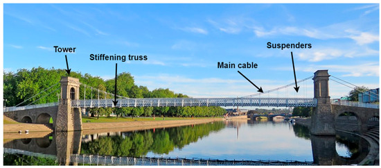
The Wilford Suspension Bridge is a double-main cable gravity-anchored footbridge over the River Trent in Nottinghamshire, England. With a span of 69 m and a width of 3.7 m, the bridge is mainly used for residents on both sides of the river and for carrying water pipes and it is composed of a steel deck covered by a floor of wooden slats, as shown in
Figure 1. The University of Nottingham has carried out several bridge structural health monitoring tests on the bridge because of its large deflections (decimeter range) under normal environmental loading. Fine finite element (FFE) analysis was carried out using the field measurement of the bridge structure size and materials
[1]. The FFE model can obtain the first three natural frequencies of the Welford Bridge, which provides a reliable and comprehensive reference for adopting the proposed method.
Figure 1. Wilford Suspension Bridge in England.
The authors carried out field tests on the suspension bridge from 15:48 to 16:30 on 31 October 2018. Two types of GNSS receivers were used in this experiment for data collection: (1) Leica GS10 GNSS geodesic receivers, whose raw observations can be sampled at a frequency of 20 Hz. It can be realized by RTK technology, horizontal 8 mm + 1 ppm, vertical 15 mm + 1 ppm, and accuracy confidence reaches more than 99.99%. (2) DM3 geodesic GNSS receivers that were manufactured by the GeoSHM team
[2], as shown in
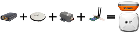
Figure 2. These receivers, as the first of their type, are also equipped with low-cost and high-precision MEMS accelerometers. The acquisition frequency of GNSS raw observations in both receivers is 20 Hz. The collected data of DM3 can obtain the same positioning accuracy and confidence interval as Leica GS10 GNSS geodesic receivers by post-processing kinematic (PPK). The sampling frequency of the accelerometer in the DM3 receiver is 100 Hz, the range is 2 g, and the acceleration noise spectrum is
0.001m/s2/Hz−−−√. In addition, supporting GNSS signal splitters, power supply, and so on are also essential.
Figure 2. DM3 geodesic GNSS/accelerometer receivers that were manufactured by the GeoSHM team. The sensor integrates a GNSS receiver, GNSS antenna, accelerometer and real-time wireless module.
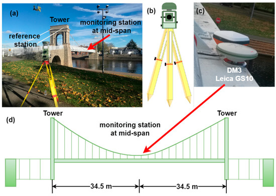
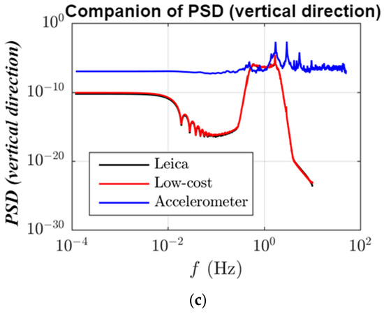
During field tests, two pairs of GS10 and DM3 receivers were placed in the quarter span and the middle span of the suspension bridge, respectively. In this experiment, the measurement information of a DM3 receiver installed in the middle position was analyzed and verified the measurement of the vibration displacement of footbridges in Nottingham (Figure 3). Another GS10 receiver is used as a reference station around 100 m away from the monitoring points, as shown in Figure 3a. The dynamic vibration of the bridge is caused by the forced vibration combined with the random vibration due to wind loading. In addition, Figure 4 shows that the power spectral densities (PSD) extracted from the GNSS measurements of both types of receivers in the three directions are very similar, indicating that the low-cost receiver fully meets the accuracy requirements of bridge structure monitoring. Therefore, in the subsequent experiments of this section, data collected with a DM3 receiver is used for analysis.
Figure 3. The Wilford Suspension Bridge in Nottingham and the instrumentation. (a) Actual locations of monitoring and reference stations; (b) reference station; (c) monitoring station (DM3 and Leica GS10) (d) the monitoring devices were fixed at the mid-span of the footbridge for dynamic response monitoring.
Figure 4. The power spectral densities (PSD) are identified by the Leica receiver (black), self-developed receiver (DM3 red), and accelerometer measurements (blue). The top left row (a) shows the PSD of longitudinal direction measurements and the top right row (b) shows the PSD of lateral direction measurements and the bottom (c) shows the PSD of vertical direction measurements.
3. Pretreatment
The data collected by GNSS and accelerometer using different coordinate systems need to be registered. The WGS84 geodetic coordinate system is used for GNSS and the accelerometer is used for the local bridge coordinate system. The WGS84 system coordinates need to be converted to the British OSGB 36NG coordinate system through the OSGM15 model. The coordinates are then converted to the bridge coordinate system by the method of plane rotation.
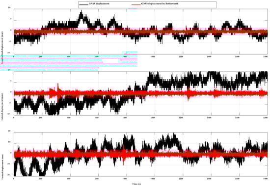
The displacement of the bridge is small and irregular due to the influence of its gravity and the underneath water pile loading. In addition, the multipath error is one of the unavoidable error sources of BSHM, which is difficult to eliminate or weaken by the empirical model or GNSS RTK. These combined effects will obscure the dynamic vibration component in the GNSS displacement time series. To reduce the interference caused by the special environment, this uses the Butterworth high-pass filter to eliminate the long-term slow displacement changes existing in the GNSS displacement time series, as shown in Figure 5.
Figure 5. GNSS displacement and dynamic vibration displacement after Butterworth at the mid−span of the Wilford Suspension Bridge. The upper row shows the results of longitudinal displacements, the middle row shows the results of lateral displacements and the bottom row shows the results of vertical displacements.
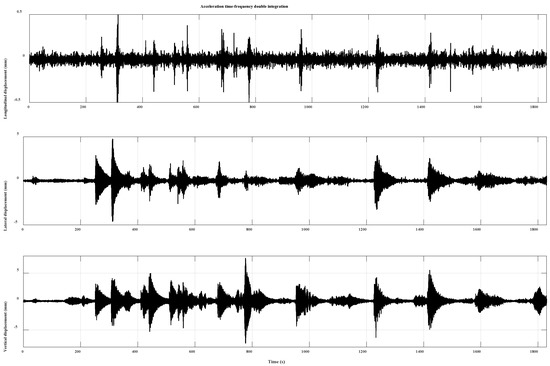
The double integral of acceleration is taken as the reference displacement. Firstly, due to the hardware delay of the data acquisition system, some epoch data are lost. The Lagrange interpolation method was used to fit the missing original acceleration data first. Secondly, the triaxial acceleration data are processed by a fifth-order Butterworth high-pass filter with a bandpass frequency of 0.2 Hz. Finally, the dynamic displacement of the bridge was obtained by time domain integration. As shown in Figure 6, the monitoring time series results of the longitudinal (along), lateral (across), and vertical axes of the bridge are respectively represented, and the results are taken as the reference truth value of this test. However, the acceleration data in the GNSS/accelerometer fusion is the original observational data that has not been processed with the Butterworth filter.
Figure 6. Displacement time series through acceleration time-frequency integration. The upper row shows the results of longitudinal displacements, the middle row shows the results of lateral displacements and the bottom row shows the results of vertical displacements.
The dynamic response of the bridge structure in the three directions can be seen from the integral result of acceleration. There is no obvious vibration and displacement deformation in the longitudinal direction, but there are apparent dynamic responses caused by forced movements in the lateral and vertical directions.
4. Robust Kalman Test for Detecting the Random Outliers of GNSS
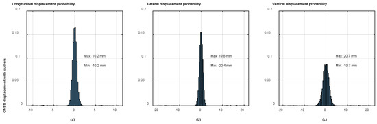
This section verifies the reliability and accuracy of the proposed method in GNSS outliers data detection. The random errors were obtained using a Gaussian-based random method with a range of (−20 mm–20 mm). These errors were then added to 1% of the time series of three-dimensional displacements. The histograms of random errors of dynamic displacements in three different directions are shown in Figure 7. The displacement has many outliers, making the distribution wider. This step is used to represent the simulation method of random outliers in GNSS displacement caused by changes in the external environment or abnormal hardware equipment. This section only shows the analysis results of part of the data from 200 s to 500 s to show the feasibility of the algorithm more clearly.
Figure 7. Histograms of random errors of dynamic displacements in three different directions. The left row (a) shows the errors of longitudinal displacements, the intermediate row (b) shows the results of lateral displacements and the right row (c) shows the results of vertical displacements.
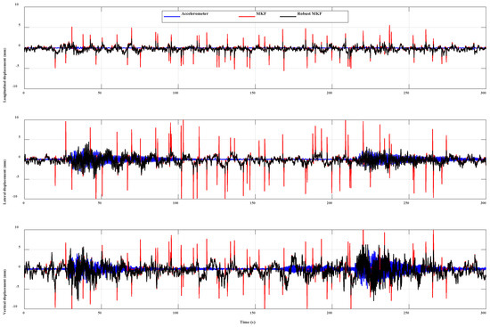
In Figure 8, 3D displacements are represented as high-precision double integral displacement of acceleration (blue), GNSS/acceleration fusion results based on the MKF method (red), and GNSS/acceleration fusion results based on the Nelder-Mead simplex RMKF (black). The RMKF method has improved both RMS, Min and Max of error combined with Table 1. The total displacement accuracy of the RMSE value has been improved by 21%. For abnormal error values, Nelder-Mead simplex RMKF has a better effect of suppressing the influence of GNSS outliers than MKF.
Figure 8. Dynamic displacements obtained in three different directions from the double integral of acceleration (blue), GNSS and accelerometer data fusion with MKF method (red), and GNSS and accelerometer data fusion with the proposed RMKF method (black). The upper row shows the results of longitudinal displacements, the middle row shows the results of lateral displacements and the bottom row shows the results of vertical displacements.
Table 1. Comparison table Mean, RMS, Max and Min error of the MKF and Robust MKF based on data of longitudinal, lateral, vertical, and total displacement.
| |
|
Mean |
RMSE |
Max |
Min |
| Longitudinal displacement |
MKF (mm) |
0.2 |
0.7 |
5.5 |
−5.6 |
| Robust MKF (mm) |
0.1 |
0.5 |
3.3 |
−2.3 |
| improved accuracy (%) |
50% |
29% |
40% |
59% |
| Lateral displacement |
MKF (mm) |
0.2 |
1.2 |
11.0 |
−10.0 |
| Robust MKF (mm) |
0.2 |
0.8 |
4.4 |
−2.8 |
| improved accuracy (%) |
- |
33% |
60% |
72% |
| Vertical displacement |
MKF (mm) |
0.4 |
1.6 |
10.8 |
−9.3 |
| Robust MKF (mm) |
0.4 |
1.4 |
5.8 |
−4.2 |
| improved accuracy (%) |
- |
13% |
46% |
55% |
| Total displacement |
MKF (mm) |
0.5 |
2.1 |
16.4 |
−14.6 |
| Robust MKF (mm) |
0.5 |
1.6 |
8.0 |
−5.5 |
| improved accuracy (%) |
- |
21% |
51% |
62% |
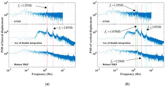
The PSD signatures of the acceleration double integration, GNSS displacements, and displacements estimated from fusing the GNSS and accelerometer data with the proposed robust RMKF method were analyzed based on the fast fourier transform (FFT) and shown in Figure 9. At the same time, it can be seen from Figure 6 above that the bridge structure has no obvious vibration in the longitudinal direction, so this only focuses on representative PSD patterns in the lateral and vertical directions.
Figure 9. Power spectral densities (PSD) of displacements from GNSS data (upper row), accelerometer measurements (middle row), and displacements from GNSS and accelerometer data fusion with the proposed RMKF method (bottom row). The left row (a) shows the results of lateral displacements and the right row (b) shows the results of vertical displacements.
Firstly, Figure 9a shows that the first mode natural frequency of 1.355 Hz and the third natural frequency of 2.855 Hz in the GNSS displacement value can be recognized, but the second mode frequency is not clear. The authors fused GNSS and acceleration data with the RMKF method to extract the second natural frequency. Figure 9b shows that GNSS data in the vertical direction did not identify the first natural frequency of 1.355 Hz because the energy of this frequency was lower than that of the second natural frequency of 1.670 Hz. For the natural frequency of 5.236 Hz, GNSS data cannot be identified. Theoretically, the sampling rate of 20 Hz of GNSS data may detect signals up to 10 Hz. However, due to the noise and outliers existing in the data during the actual observation, the modal frequency of 5.236 Hz has been buried in it, and it cannot be identified through spectral analysis. In contrast, the accelerometer data and the combination of GNSS and accelerometer data capture the frequency well.
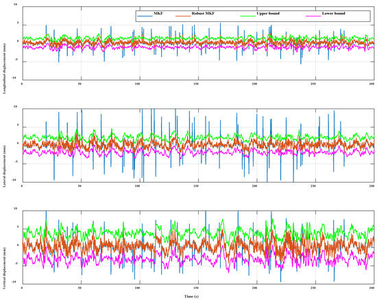
The advantage of the RMKF is also demonstrated by comparing alarm thresholds. During the field experimenters, a large number of jumping or running situations were executed, resulting in large dynamic vibration of the bridge in the experiment. Therefore, it is unscientific to use a fixed threshold to monitor the displacement and to give an alarm when the threshold is exceeded. The alarm threshold interval is mainly divided into three steps. First, the double integral dynamic displacement of the accelerometer with noise reduction is used as a reference. Then the error-free GNSS/acceleration fusion displacement is distinguished from the reference. Finally, three times the standard deviations (STD) are constructed as the threshold range, as shown in Figure 10. If the residual difference between the obtained displacement and the reference value exceeds the threshold range, it is judged as an alarm situation. After Nelder-Mead simplex RMKF treatment, the influence of GNSS outliers is effectively weakened, so that their displacement is below the threshold, and there is no error alarm. However, the displacements (with many blue spikes) processed by conventional MKF still exceed the threshold, which will affect the assessment of structural conditions, and in this case, the false alarm rate reaches 92%. Therefore, the RMKF method can effectively improve the accuracy of the alarm system and greatly reduce the false alarm caused by these gross errors.
Figure 10. Spatiotemporal warning of dynamic displacement error. The upper row shows the results of l longitudinal displacements, the middle row shows the results of lateral displacements and the bottom row shows the results of vertical displacements.
This entry is adapted from the peer-reviewed paper 10.3390/rs15092385