Your browser does not fully support modern features. Please upgrade for a smoother experience.
Please note this is an old version of this entry, which may differ significantly from the current revision.
Advances in artificial intelligence (AI), especially deep learning (DL), have facilitated magnetic resonance imaging (MRI) data analysis, enabling AI-assisted medical image diagnoses and prognoses. However, most of the DL models are considered as “black boxes”. There is an unmet need to demystify DL models so domain experts can trust these high-performance DL models. This has resulted in a sub-domain of AI research called explainable artificial intelligence (XAI).
- deep learning
- explainable artificial intelligence
- magnetic resonance imaging
1. Introduction
Advances in artificial intelligence (AI), especially deep learning (DL), have enabled more complex magnetic resonance imaging (MRI) data analysis, facilitating tremendous progress in automated image-based diagnoses and prognoses [1]. Previously, medical image analyses were typically performed using systems fully designed by human domain experts [2]. Such an image analysis system could be a statistical or machine learning (ML) model that used handcrafted properties (i.e., image features) of an image or regions of interest (ROIs) on the image [3]. These handcrafted image features range from low-level (e.g., edges or corners) to higher-level image properties (e.g., texture). Modern DL models can automatically learn these image features with minimal human interference to optimally perform certain image analysis tasks, which improves efficiency and saves a lot of human resources [4]. The fast development of DL has contributed to its growing application in MRI image analysis.
Due to their non-linear underlying structures, most DL models are considered as “black boxes” by scholars, and even more so by the public [5]. There is an urgent need for more tools to demystify these DL models, which has resulted in a sub-domain of AI research called explainable artificial intelligence (XAI). The emergence of XAI has mainly been driven by three factors: (a) the need to increase the transparency of AI models; (b) the necessity to allow humans to interact with AI models; and (c) the requirement for the faithfulness of their inferences. The above reasons have led to the rapid development of domain-dependent and context-specific techniques when dealing with the interpretation of DL models and the formation of explanations for public understanding [6]. Recently, many experts have dedicated their efforts to developing novel methods that are competent at visualizing and explaining the logic behind data-driven DL models.
2. Overview of MRI Images
MRI uses the principle of nuclear magnetic resonance (NMR) [7] and maps the internal structure of an object by acquiring the position and type of its atomic nuclei [8]. The application of gradient magnetic fields leads to the emission of electromagnetic waves based on the attenuation of the energy released in different structural environments within a substance. As a noninvasive imaging technology, MRI can produce high-quality images without the use of ionizing radiation. Thus, MRI can safely provide a wealth of diagnostic information, which makes medical diagnoses and functional studies of the human body convenient and effective [9]. MRI is a versatile medical imaging technique that produces images of organs, tissues, bones, and other structures for a range of medical conditions, and has been widely used in clinical disease screening, diagnosis, treatment guidance, and evaluation since the mid-1980s. Figure 2 illustrates a number of examples using different MRI techniques from various human organs. In this section, the researchers will review a few common MRI techniques that have been widely utilized in both the clinical and research domains.
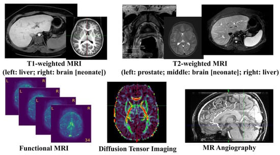
Figure 2. Illustration of common MRI Images.
2.1. Anatomical MRI
T1-weighted MRI is one of the most commonly used anatomical MRI sequences using T1 relaxation time [8]. T1 (also known as spin–lattice or longitudinal) relaxation time is the time for the z component of a spin to return to 63% of its original position following a radiofrequency (RF) excitation pulse. Since various tissues require different T1 relaxation times to return to equilibrium, one can highlight the tissues’ contrast using differences in the T1 relaxation times. T2-weighted MRI is another common anatomical MRI sequence, which relies on T2 relaxation time [10]. T2 (also known as spin–spin or transverse) relaxation time is the time required for the transverse component of a proton to decay to 37% of its initial status through irreversible processes [8]. Similar to T1-weighted MRI, various human tissues also have different T2 relaxation times, so the researchers can demonstrate the tissues’ contrast using differences in the T2 relaxation times. T1-weighted images are produced by scans using short Time to Echo (TE) time and Repetition Time (TR). Conversely, T2-weighted images are generated by scans using longer TE and TR time. The contrast and brightness of anatomical MRI images are predominately determined by the T1 and T2 properties of the tissue, separately. While T1-weighted images tend to have a high-signal intensity on fat and low intensity on water, T2-weighted images have an intermediate–high-signal intensity on fat and high intensity on water. For example, T1-weighted MRI images highlight white matter for the adult brain, while T2 MRI images highlight cerebrospinal fluid and inflammation [11].
2.2. Diffusion MRI
Diffusion MRI, or diffusion-weighted imaging (DWI), is one MRI technique that generates image contrast by measuring the Brownian motion of the water molecules within tissues. Diffusion Tensor Imaging (DTI), a special type of DWI, is one of the most popular diffusion MRI techniques in brain research and clinical practice for mapping white matter tractography [12]. It measures the diffusion anisotropy of water molecules traveling in white matter fibers, where a higher speed is observed in parallel motion compared to perpendicular movements. By detecting the variations in the signals from hydrogen atoms, DTI can capture the orientations of the white matter tracts in the brain. Quantitative diffusion metrics, such as fractional anisotropy, axial diffusivity, mean diffusivity, and radial diffusivity, have been extensively used in brain research to reveal the white matter integrity. These white matter tracts have found multiple neuroimaging applications, such as brain structural and functional mapping, evaluations of brain injury, disease progression, surgical planning, and treatment response monitoring [13].
2.3. Functional MRI (fMRI)
Functional MRI (fMRI) is an imaging technique measuring the time-varying brain activity reflected by the fluctuations of blood oxygen levels caused by brain metabolism [14]. The oxygen is believed to concentrate at the location where the neural activity is highly active. Due to the magnetic sensitivity difference between the oxygenated and deoxygenated hemoglobin, a measurable signal is detected by the MRI scanner. Two types of brain activation patterns can be obtained when subjects are in a resting state (resting state fMRI) or taking on targeted tasks (task fMRI). Since fMRI data are 4D time-varying volume data, graph-based approaches are widely used to construct the brain’s functional connectomes from the fMRI data by estimating the correlations between the distinct brain regions, where each node represents a brain region and the edges represent the functional connections. In recent years, fMRI has been used to investigate a wide range of cognitive tasks, including attention, emotion, working memory, language, and decision making, as well as neurological and psychiatric disorders (e.g., Alzheimer’s disease, attention deficit hyperactivity disorder, and schizophrenia).
2.4. Magnetic Resonance Angiography (MRA)
Magnetic resonance angiography (MRA) [15] is a special type of MRI designed to image the vascular system. It plays an essential role in the accurate diagnosis of and treatment selection for patients with arterial disease. Contrast-enhanced (CE) MRA provides more detailed images for more precise diagnoses with shorter acquisition times and reduced artifacts caused by blood flow and pulsatility, but increases examination expenses and the risk of nephrogenic systemic fibrosis caused by gadolinium-based agents. Non-contrast-enhanced (NCE) MRA provides a safer tool for generating image contrasts between blood vessels and background tissues and is becoming increasingly popular in clinical practice. Among the various NCE MRA techniques, time-of-flight (TOF) imaging is the most common and is widely used in clinical practice and research fields [16], which measures the magnetization state difference between stationary tissues and blood flow. TOF MRA has been applied to the assessment, diagnosis, and treatment of multiple cerebrovascular and arterial diseases.
3. Brief Introduction of AI Models
Multi-layer perceptron (MLP), also known as artificial neural networks, are one of the most classic ML models [17]. An MLP consists of an input layer, many hidden layers in the middle, and an output layer. Each neuron in an MLP is connected to all the nodes in the previous layer. Since MLPs have a large number of weights in each layer, it is difficult to train these models, especially when the data dimension (such as images) is high. Additionally, as MLPs only accept vectorized features as inputs, they are not a preferrable model for image data that contain spatial information. More recently, deep neural networks (DNN) have been commonly utilized to refer to MLP models with a large number of hidden layers.
Convolutional neural networks (CNN) are the most frequently utilized models for tackling different medical imaging tasks, such as image classification/regression. Different from the fully connected neurons in MLPs or DNNs, CNN models rely on shared local trainable kernels/filters to perform their image convolution operations on the input images to extract the image features. Compared to MLP models, CNN models not only incorporate the spatial location of the shared features within the input data/images, but also have a decreased computational complexity, resulting in less encoding of the overall parameters [18]. Taken together, these characteristics open up the possibility for the application of CNN models to more limited, sparse datasets, as seen in the setting of medical imaging applications. A major milestone in DL history is AlexNet [19], a CNN model that won the ImageNet competition in 2012 with outstanding scores. Since then, multiple CNN models, such as the Visual Geometry Group (VGG) [20], GoogLeNet [21], and Residual Networks (ResNet) [22], have been developed to further improve the capability of image classification and recognition.
For image segmentation, U-Net [23] or its variations become desirable DL models. The principle of U-Net is to use a U-shaped CNN architecture with skip connections to compute attention maps at full input resolution to help in the detection of small objects. More specifically, U-Net, as well as its variation models (e.g., V-Net and ResU-Net), all consist of a contracting path and an expanding path. Each path has the repeated block of convolutional/deconvolutional layers, non-linear activation layers, and pooling layers for feature learning and reconstruction.
Graph neural networks (GNN) [24] generalize DL models on graph-based data. As the most classical and widely used GNN, a graph convolutional network (GCN) [25] has been proposed by Kipf and Welling as an efficient variant of a CNN that performs convolution on graphs. Various variants of GNN models, such as the Graph Isomorphism Network (GIN) [26], Graph Attention Network (GAT) [27], and GraphSAGE [28], have been proposed and adopted to tackle medical image problems at the node level, edge level, and graph level.
This entry is adapted from the peer-reviewed paper 10.3390/diagnostics13091571
References
- Mazurowski, M.A.; Buda, M.; Saha, A.; Bashir, M.R. Deep learning in radiology: An overview of the concepts and a survey of the state of the art with focus on MRI. J. Magn. Reson. Imaging 2019, 49, 939–954.
- Dhawan, A.P. Medical Image Analysis; John Wiley & Sons: Hoboken, NJ, USA, 2011.
- Phillips, J.J. ROI: The search for best practices. Train. Dev. 1996, 50, 42–48.
- Suzuki, K. Overview of deep learning in medical imaging. Radiol. Phys. Technol. 2017, 10, 257–273.
- Castelvecchi, D. Can we open the black box of AI? Nat. News 2016, 538, 20.
- Vilone, G.; Longo, L. Classification of Explainable Artificial Intelligence Methods through Their Output Formats. Mach. Learn. Knowl. Extr. 2021, 3, 615–661.
- Günther, H. NMR Spectroscopy: Basic Principles, Concepts and Applications in Chemistry; John Wiley & Sons: Hoboken, NJ, USA, 2013.
- Dale, B.M.; Brown, M.A.; Semelka, R.C. MRI: Basic Principles and Applications; John Wiley & Sons: Hoboken, NJ, USA, 2015.
- Filippi, M.; Rocca, M.A.; Ciccarelli, O.; De Stefano, N.; Evangelou, N.; Kappos, L.; Rovira, A.; Sastre-Garriga, J.; Tintorè, M.; Frederiksen, J.L. MRI criteria for the diagnosis of multiple sclerosis: MAGNIMS consensus guidelines. Lancet Neurol. 2016, 15, 292–303.
- Young, G.S. Advanced MRI of adult brain tumors. Neurol. Clin. 2007, 25, 947–973.
- Plewes, D.B.; Kucharczyk, W. Physics of MRI: A primer. J. Magn. Reson. Imaging 2012, 35, 1038–1054.
- Assaf, Y.; Pasternak, O. Diffusion tensor imaging (DTI)-based white matter mapping in brain research: A review. J. Mol. Neurosci. 2008, 34, 51–61.
- Tae, W.S.; Ham, B.J.; Pyun, S.B.; Kang, S.H.; Kim, B.J. Current Clinical Applications of Diffusion-Tensor Imaging in Neurological Disorders. J. Clin. Neurol. 2018, 14, 129–140.
- Glover, G.H. Overview of functional magnetic resonance imaging. Neurosurg. Clin. N. Am. 2011, 22, 133–139.
- Hartung, M.P.; Grist, T.M.; François, C.J. Magnetic resonance angiography: Current status and future directions. J. Cardiovasc. Magn. Reson. 2011, 13, 19.
- Shin, T. Principles of Magnetic Resonance Angiography Techniques. Investig. Magn. Reson. Imaging 2021, 25, 209–217.
- Riedmiller, M. Advanced supervised learning in multi-layer perceptrons—from backpropagation to adaptive learning algorithms. Comput. Stand. Interfaces 1994, 16, 265–278.
- Chua, L.O.; Roska, T. The CNN paradigm. IEEE Trans. Circuits Syst. I Fundam. Theory Appl. 1993, 40, 147–156.
- Krizhevsky, A.; Sutskever, I.; Hinton, G.E. Imagenet classification with deep convolutional neural networks. Commun. ACM 2017, 60, 84–90.
- Simonyan, K.; Zisserman, A. Very deep convolutional networks for large-scale image recognition. arXiv 2014, arXiv:1409.1556.
- Szegedy, C.; Liu, W.; Jia, Y.; Sermanet, P.; Reed, S.; Anguelov, D.; Erhan, D.; Vanhoucke, V.; Rabinovich, A. Going deeper with convolutions. In Proceedings of the IEEE Conference on Computer Vision and Pattern Recognition, Boston, MA, USA, 7–12 June 2015; pp. 1–9.
- He, K.; Zhang, X.; Ren, S.; Sun, J. Deep residual learning for image recognition. In Proceedings of the IEEE Conference on Computer Vision and Pattern Recognition, Las Vegas, NV, USA, 27–30 June 2016; pp. 770–778.
- Ronneberger, O.; Fischer, P.; Brox, T. U-net: Convolutional networks for biomedical image segmentation. In Proceedings of the Medical Image Computing and Computer-Assisted Intervention—MICCAI 2015: 18th International Conference, Munich, Germany, 5–9 October 2015; Part III 18. pp. 234–241.
- Zhou, J.; Cui, G.; Hu, S.; Zhang, Z.; Yang, C.; Liu, Z.; Wang, L.; Li, C.; Sun, M. Graph neural networks: A review of methods and applications. AI Open 2020, 1, 57–81.
- Kipf, T.N.; Welling, M. Semi-supervised classification with graph convolutional networks. arXiv 2016, arXiv:1609.02907.
- Xu, K.; Hu, W.; Leskovec, J.; Jegelka, S. How powerful are graph neural networks? arXiv 2018, arXiv:1810.00826.
- Velickovic, P.; Cucurull, G.; Casanova, A.; Romero, A.; Lio, P.; Bengio, Y. Graph attention networks. Stat 2017, 1050, 10–48550.
- Hamilton, W.; Ying, Z.; Leskovec, J. Inductive representation learning on large graphs. In Proceedings of the Advances in Neural Information Processing Systems 30: Annual Conference on Neural Information Processing Systems 2017, Long Beach, CA, USA, 4–9 December 2017.
This entry is offline, you can click here to edit this entry!