Your browser does not fully support modern features. Please upgrade for a smoother experience.
Please note this is an old version of this entry, which may differ significantly from the current revision.
Subjects:
Engineering, Aerospace
Safety critical spare parts hold special importance for aviation organizations. However, accurate forecasting of such parts becomes challenging when the data are lumpy or intermittent. Different methods, with varying degrees of success, have been used to forecast lumpy and intermittent demand data.
- lumpy demand forecasting
- aviation
- machine learning
- spare part demand prediction
1. Introduction
Safety is the most desired feature for aviation, and safety critical spare parts hold special importance for aviation organizations. Forecasting future consumption of safety-related spare parts is the most critical part of inventory management, as its inaccurate prediction poses a serious challenge for the organizations responsible for the maintenance of aviation fleets [1]. Keeping in view efficient spare parts management and decreasing maintenance budget, possession of a reasonable inventory level is critical in the aviation industry, where lead time does not always satisfy the actual demand due to which spare parts pile up in the warehouse. Figure 1 provides an example of a sample depot that is responsible for the storage of spares and for the maintenance of helicopters and fixed-wing aircraft from four different origins. The depot stores around 97,693 spares, including 18,930 time change components (TBOs) that are categorized as slow-moving spares. These spares are expensive and are replaced based on either operational time or calendar years. The depot maintains two types of spares—fast-moving spares (selective stock list (SSL) and expandable spares) and slow-moving spares (TBOs, and non-selective stock list (nonSSL)). The SSL items are stocked for one quarter based on the demand/consumption of the previous four quarters. The TBOs, being critical and costly items, are stored for the next five years, based on the last two years of consumption data from maintenance setups. NonSSL and expandable items are stored for four quarters based on projections.
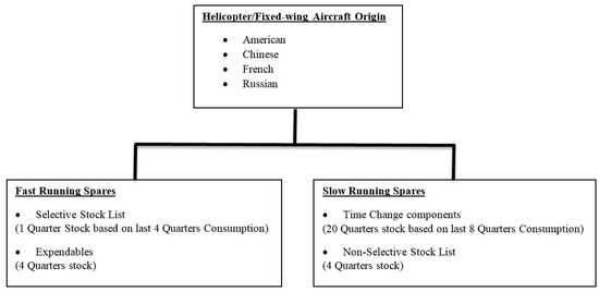
Figure 1. A sample spare depot storage template.
The problem of modeling future consumption is further aggravated by a lumpy spare part demand pattern [2,3], marked by periods with no demand along with sporadic demand [4,5], as shown in Figure 2.
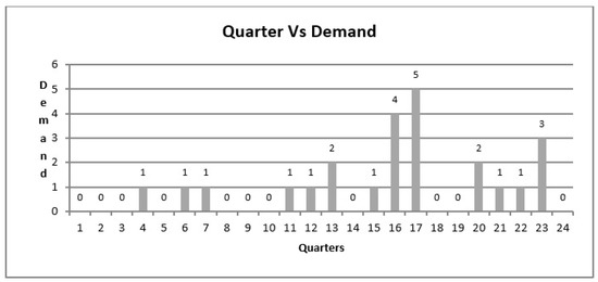
Figure 2. Lumpy demand forecasting graphical representation.
The continuous inspections and preventive maintenance render the aircraft unserviceable for operational requirements, which costs the maintenance organizations. Therefore, the topmost priority for small and medium enterprises is to make the right spare parts available at the need of the hour and at the required location. The increasing downtime of the aircraft can be managed with efficient forecasting to have better operational fleet performance, which is a less researched domain in the aviation sector and warrants investigation. In this connection, the system experts [6,7] have utilized the statistical techniques of exponential smoothing and regression analysis [8,9], but such approaches are found to perform inaccurately when a lumpy demand pattern is processed [10]. Another interesting approach presents an innovative model for a single site to take advantage of a distribution, the zero-inflated Poisson. The researchers demonstrate the model effectiveness, confirming that their approach outperforms the traditional Poisson-based approach [11].
Different methods, with varying degrees of success, have been used to forecast lumpy and intermittent demand data. These techniques comprise a variety of models, such as Holt–Winterss [12] as the statistical method. Similarly, machine learning methods such as the support vector regression (SVR) [13] are used, while long short-term memory (LSTM) networks [14] are used as a deep learning method. However, it is still debatable which technique or meta-level approach predicts lumpy and intermittent demand data most accurately. This is due to a lack of historical research on intermittent and lumpy time series data [15]. In recent years, machine learning and deep learning research has also advanced rapidly.
Among these, artificial neural networks (ANN) are considered the most recognized artificial intelligence (AI) method [16] used to handle lumpy demand patterns because they have outperformed the traditional techniques in several fields [17,18,19,20]. Owing to the added advantage of performing in the way the human brain works by acquiring training from historical demand data, such models perform superbly. Afterward, they infer future demand based on the nonlinear pattern recognition and correlation establishment between the predictor variables and the outcomes. This way of learning has attracted many system managers in the field of aviation to harness the uncertainties and to solve future spare parts demand. On the other hand, the limitation to the use of ANN remains, as it is difficult to explore the best forecasting model because of the sensitivity analysis requirement on learning rate, momentum coefficient, and the number of hidden neurons.
2. Spare Parts Forecasting and Lumpiness Classification Methods
John Croston was the first to introduce a method that was designed specifically for intermittent data [21]. Croston proposed separating the data into two series: one for arrival times and another for positive demand. Croston noted, however, that the time series data for intermittent demand varied significantly from that of conventional time series data. The former have multiple zero-demand intervals that are different from the latter. He presented an alternative technique to forecast demand from intermittent time series data. Croston stated that his method that presupposes independence between demand size and demand intervals. However, Willemain et al. [22] casted doubt on this concept of autonomy. This, however, was maintained in subsequent work that improved Croston’s original method, such as Syntetos and Boylan [23]. Syntetos and Boylan investigated Croston’s method and found it to be biased. Later, they presented a modified version of Croston’s method to resolve the bias issue [24].
Leve’n and Segerstedt proposed a modification of Croston’s technique that attempts to eliminate its inherent bias [8]. Nevertheless, the Leve’n and Segerstedt method is more biased than the Croston method, particularly for highly intermittent series. Willemain et al. identified patterns of intermittent demand in several other scenarios such as heavy machinery, electronics, maritime spare parts, etc. [25]. Similarly, Syntetos and Boylan studied intermittency in automotive spare parts [26]. Ghobbar and Friend analyzed the demand for costly aircraft maintenance parts [1]. They observed that businesses were holding too much inventory due to inaccurate demand forecasts, resulting in subpar service levels. Whether the demand is large or small or arrives at the correct or incorrect time, both can lead to mistakes. Therefore, accurate demand projections are necessary to support inventory holding and replenishment decisions. In addition, as a result of shortened life cycles, technology migrations, time for lengthy production cycles, and protracted lead times for capacity expansion, electronic companies face complexity in inventory management and risk of excess supply and shortfall of important components [27].
The work of [28] performs intermittent prediction on data collected from the Internet of things (IoT) using a recurrent neural network (RNN). The performance evaluation metric is accuracy. In this specific prediction task, RNNs outperformed ANNs. As an alternative to the Croston method, a new method based on stochastic simulation is used to conduct research in [29]. Different evaluation metrics are used such as mean error (ME), mean absolute deviation (MAD), MASE, and D proposed by the authors. In conclusion, the proposed method did not outperform the existing standard. In [30], the ATA technique was compared with the Croston technique. The data from the M4 competition were utilized. The ATA and the exponential smoothing methods are similar, but their respective emphases differ. The study predicted six future time steps. As evaluation metrics, both mean squared error and standardized mean absolute percentage error are utilized. As a metric for out-of-sample evaluation, the ATA method is superior to the Croston method. In [31], a novel method, the modified SBA, is presented for intermittent forecasting. In conclusion, the proposed method can not compete with the current method. The authors of [32] employ a deep neural network (DNN) to predict sensor data. The ARIMA and generalized autoregressive conditional heteroskedasticity (GARCH) techniques have been surpassed by this method. It utilized simulations that require a well-considered parameter design for this purpose. Ref. [33] provides an example of a simulation design that investigates multiple parameter combinations. The study results demonstrate promising outcomes.
A study in [34] introduces a seasonal adjustment method and a dynamic neural network as the primary seasonal forecasting model. Zero demand is counteracted by preprocessing the initial input data and by adding input nodes to the neural network. It proposed a revised error measurement method for evaluating performance. The proposed framework for forecasting outperforms competing models for intermittent demand. Two ANN models, each using 36 observations as training data, were proposed in [35]. The proposed model was able to achieve competitive inventory performance relative to Croston despite low forecasting accuracy. In [36], an ANN and RNN are trained and compared for intermittent demand forecasting. The results show that ANN performance is superior to that of RNN in long-term demand series. Another work in [37] conducts an empirical analysis utilizing 5133 SKUs from an airline and acquired forecast performance and inventory performance outcomes for different methodologies. The findings indicate that proposed ANN approaches are less biased as compared to other evaluated methods.
Table 1 summarizes different datasets having different patterns including intermittent, lumpy, and smooth. It also shows the industry related to each dataset. The forecasting methods used in the referenced article and its evaluated metrics are also included. From the table, it can be observed that the performance of various methods varies with the input datasets.
Table 1. Datasets having intermittent lumpy and smooth patterns, their forecasting methods, and accuracies on different metrics. The ’×’ indicates that the value for this parameter is not reported.
| Series Type | Ref. | Application | Forecasting Method | MAE | sMAPE | RMSE | MAD | MASE |
|---|---|---|---|---|---|---|---|---|
| Intermittent | 2021 [38] | Retail industry | SBA | × | × | 0.632 | × | × |
| SES | × | × | 0.617 | × | × | |||
| Croston | × | × | 0.630 | × | × | |||
| Markov-combined method | 0.328 | 0.406 | 0.576 | × | × | |||
| 2019 [27] | Electronics distribution | ARIMA | 12.39 | × | 16.90 | × | 1.108 | |
| Croston | 13.24 | × | 17.31 | × | 1.197 | |||
| SVM | 10.11 | × | 16.72 | × | 0.901 | |||
| RNN | 9.29 | × | 16.61 | × | 0.792 | |||
| UNISON data driven | 9.19 | × | 15.13 | × | 0.768 | |||
| 2021 [39] | Vehicle industry | SVM | × | × | × | × | 0.830 | |
| ANN | × | × | × | × | 0.954 | |||
| RNN | × | × | × | × | 0.999 | |||
| 2017 [40] | Naval industry | SES | × | × | × | × | 1.796 | |
| SBA | × | × | × | × | 1.678 | |||
| TSB | × | × | × | × | 1.700 | |||
| Bootstrap | × | × | × | × | 1.981 | |||
| LUMPY | 2021 [39] | Vehicle industry | SVM | × | × | × | × | 0.821 |
| ANN | × | × | × | × | 1.042 | |||
| RNN | × | × | × | × | 1.069 | |||
| 2005 [41] | Space industry | SES | × | × | × | 9.26 | × | |
| Croston | × | × | × | 8.77 | × | |||
| 2008 [21] | Electronics | SBA | × | 138.36 | × | × | × | |
| NN | × | 128.20 | × | × | × | |||
| SMOOTH | 2021 [39] | Vehicle industry | SVM | × | × | × | × | 0.877 |
| ANN | × | × | × | × | 0.930 | |||
| RNN | × | × | × | × | 0.987 | |||
| 2020 [42] | Furniture industry | ARIMA | × | 0.1616 | 3531 | × | × | |
| KNN | × | 0.1374 | 2913 | × | × | |||
| RNN | × | 0.1333 | 2788 | × | × | |||
| ANN | × | 0.1011 | 2115 | × | × | |||
| SVM | × | 0.1101 | 1967 | × | × | |||
| LSTM | × | 0.1072 | 2267 | × | × | |||
| Dilated LSTM | × | 0.1023 | 2172 | × | × | |||
| 2021 [43] | Electric power | ANN | × | 5.27 | 378 | × | × | |
| ARIMA | × | 5.65 | 463 | × | × | |||
| GRNN | × | 5.01 | 350 | × | × | |||
| LSTM | × | 6.11 | 431 | × | × | |||
| ETS+RD-LSTM | × | 4.46 | 351 | × | × |
This entry is adapted from the peer-reviewed paper 10.3390/app13095475
This entry is offline, you can click here to edit this entry!