Your browser does not fully support modern features. Please upgrade for a smoother experience.
Please note this is an old version of this entry, which may differ significantly from the current revision.
Deep learning models, specifically convolutional neural networks (CNNs), are well known for understanding images. An artificial neural network (ANN) is an algorithm based on interconnected nodes to recognize the relationships in a set of data. Algorithms based on ANNs have shown a great success in modeling both the lineßar and the non-linear relationships in the underlying data. Due to the huge success rate of these algorithms, they are extensively being used for different real-time applications.
- automatic video classification
- deep learning
- handcrafted features
- video processing
1. Convolutional Neural Networks (CNN) for Image Analysis
Deep learning models, specifically convolutional neural networks (CNNs), are well known for understanding images. A number of CNN architectures are proposed and developed in the scientific literature for image analysis. Among these, the most popular architectures are LeNet-5 [1], AlexNet [2], VGGNet [3], GoogleNet [4], ResNet [5], and DenseNet [6]. The trend that follows from the formerly proposed architectures towards the recently proposed architectures is to deepen the network. A summary of these popular CNN architectures along with trend of deepening the network is shown in Figure 1, where the depth of network increases from left-most (LeNet-5) to right-most (DenseNet). Deep networks are believed to better approximate the target function and to generate better feature representation with more powerful discriminatory powers [7]. Although deeper networks are better in terms of having more discriminatory powers, the deeper networks require more data for training and more parameters to tune [8]. Finding a professionally labeled, huge dataset is still a big challenge faced by the research community, and therefore, it limits the development of deeper neural networks.
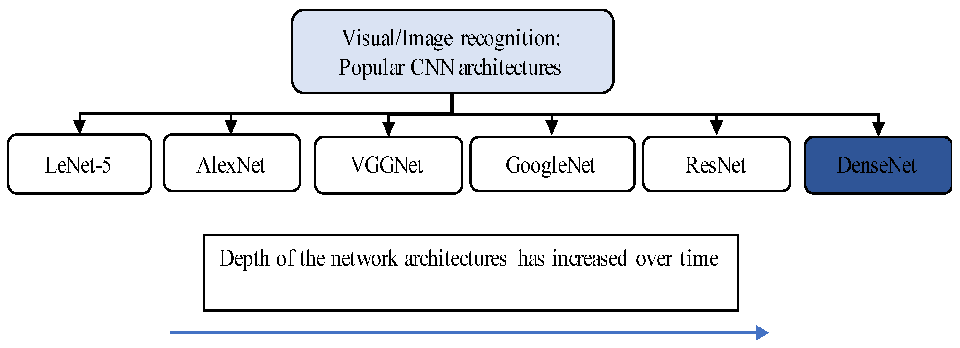
Figure 1. State-of-art image recognition CNN networks. The trend is that the depth and discriminatory powers of network architectures increases from formerly proposed architectures towards the recently proposed architectures.


2. Video Classification
2.1. Video Data Modalities
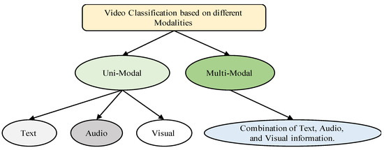
As compared to images, videos are more challenging to understand and classify due to the complex nature of the temporal content. However, three different modalities, i.e., visual information, audio information, and text information, might be available to classify videos in contrast to image classification, where only a single visual modality can be utilized. Based on the availability of different modalities in videos, the task of classification can be categorized as a uni-modal video classification or a multi-modal video classification, as summarized in Figure 2.

Figure 2. Different modalities used for classification of videos.
2.2. Traditional Handcrafted Features
During the earlier developments of the video classification task, the traditional handcrafted features were combined with state-of-art machine learning algorithms to classify the videos. Some of the most popular handcrafted feature representation techniques used in the literature are spatiotemporal interest points (STIPs) [9], improved dense trajectories (iDT) [10], SIFT-3D [11], HOG3D [12], motion boundary histogram [13], action-bank [14], cuboids [15], 3D SURF [16], and dynamic-poselets [17]. These hand-designed representations use different feature encoding schemes such as the ones based on pyramids and histograms. iDT is one of these handcrafted representations that is widely considered the state-of-the-art. Many recent competitive studies demonstrated that handcrafted features [18][19][20][21] and high-level [22][23] and mid-level [24][25] video representations have contributed towards the task of video classification with deep neural networks.
2.3. Deep Learning Frameworks
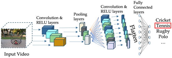
Along with the development of more powerful deep learning architectures in the recent years, the trend for the video classification task has followed a shift from traditional handcrafted approaches to the fully automated deep learning approaches. Among the very common deep learning architectures used for video classification is a 3D-CNN model. An example of 3D-CNN architecture used for video classification is given in Figure 3 [26]. In this architecture, 3D blocks are utilized to capture the video information necessary to classify the video content. One more very common architecture is a multi-stream architecture, where the spatial and temporal information is separately processed, and the features extracted from different streams are then fused to make a decision. To process the temporal information, different methods are used, and the two most common methods are based on (i) RNN (mainly LSTM) and (ii) optical flow. An example of a multi-stream network model [27], where the temporal stream is processed using optical flow, is shown in Figure 4. A high-level overview of the video classification process is shown in Figure 5, where the stages of feature extraction and prediction are shown with the most common type of strategies used in the literature. In the upcoming sections, the breakthroughs in video classification and studies related to classification of videos, specifically using deep learning frameworks, are summarized, describing the success rate of utilizing deep learning architectures and the associated limitations.

Figure 3. An example of 3D-CNN architecture to classify videos.

Figure 4. An example of two-stream architecture with optical flow.

Figure 5. An overview of video classification process.
2.4. Breakthroughs
The breakthroughs in recognition of still-images originated with the introduction of a deep learning model called AlexNet [2]. The same concept of still-image recognition using deep learning is also extended for videos, where individual video frames are collectively processed as images by a deep learning model to predict the contents of a video. The features from individual video frames are extracted, and then, temporal integration of such features into a fixed-size descriptor using pooling is performed. The task is either done using high-dimensional feature encoding [28][29] or through the RNN architectures [30][31][32][33].
2.5. Basic Deep Learning Architectures for Video Classification
The two most widely used deep learning architectures for video classification are convolutional neural network (CNN) and recurrent neural network (RNN). CNNs are mostly used to learn the spatial information from videos, whereas RNNs are used to learn the temporal information from videos, as the main difference between these two architectures is the ability to process temporal information or data that come in sequences. Therefore, both these network architectures are used for completely different purposes in general. However, the nature of video data with the presence of both the spatial and the temporal information demands the use of both these network architectures to accurately process the two-stream information. The architecture of a CNN applies different filters in the convolutional layers to transform the data. RNNs, on the other hand, reuse the activation functions to generate the next output in a series from the other data points in the sequence. However, the use of only 2D-CNNs alone limits the understanding of video to only spatial domain. RNNs, on the other hand, can understand the temporal content of a sequence. Both these basic architectures and their enhanced versions are applied in several studies for the task of video classification.
2.6. Developments in Video Classification over Time
The trend observed for the classification of videos from the existing literature is that the recently developed state-of-art deep learning models are outperforming the earlier handcrafted classical approaches. This is mainly due to the availability of large-scale video data for learning deep architectures of neural networks. Besides an improvement in classification performance the recently developed models are mostly self-learned and does not require any manual feature engineering. This added advantage makes them more feasible for use in real applications. However, the better performing recently developed architectures are deeper as compared to the previously developed architectures which brings a compromise on the computational complexity of the deep architectures.
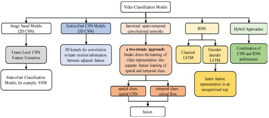
The development of 3D-CNN models paved the way for fully automatic video classification models using different deep learning architectures. Among the developments using deep learning architectures, spatiotemporal convolutional networks are approaches based on integration of temporal and spatial information using convolutional networks to perform video classification. To collect temporal and spatial information, these methods primarily rely on convolution and pooling layers. Stack optical flow is used in two/multi-stream networks methods to identify movements in addition to context frame visuals. Recurrent spatial networks use recurrent neural networks (RNN) to model temporal information in videos, such as LSTM or GRU. The ResNet architecture is used to build mixed convolutional models. They are particularly interested in models that utilize 3D convolution in the bottom or top layers but 2D in the remainder; these are referred to as “mixed convolutional” models. These also include methods based on mixed temporal convolution with different kernel sizes. Advanced architectures based on DenseNet have also shown promising results for the video classification task. Some of these notable architectures based on DenseNet include region-based CNN (R-CNN) [34][35], faster R-CNN [36][37], and YOLO [38]. Besides these architectures, there are also hybrid approaches based on the integration of CNN and RNN architectures. A summary of these architectures is provided in Figure 6.

Figure 6. Summary of video classification approaches.
2.7. Few-Shot Video Classification
FEW-SHOT learning (FSL) has received a great deal of interest in recent years. FSL tries to identify new classes with one or a few labeled samples [39][40][41][42]. However, due to most recent work in few-shot learning being centered on image classification, FSL in the video domain is still hardly being explored [43][44]. Some of the notable works done in this domain are discussed below.
A multi-saliency embedding technique was developed by Zhu et al. [44] to encode a variable-length video stream into a fixed-size matrix. Graph neural networks (GNN) were developed by Hu et al. [45] to enhance the video classification model’s capacity for discrimination. The local–global link in a distributed representation space was still disregarded nevertheless. To categorize a previously unseen video, Cao et al. [46] introduced a temporal alignment module (TAM) that explicitly took advantage of the temporal ordering information in video data through temporal alignment.
2.8. Geometric Deep Learning
Shape descriptors play a significant role in the description of manifolds for 3D shapes. In general, a global feature descriptor is created by aggregating local descriptors to describe the geometric properties of the entire shape, for example, using the bag-of-features paradigm. A local feature descriptor assigns a vector to each point on the shape in a multi-dimensional descriptor space, representing the local structure of the shape around that point. Most deep learning techniques that deal with 3D shapes essentially use the CNN paradigm. Volumetric 2D multi-view shape representations are applied directly using standard (Euclidean) CNN architectures in neural networks via methods such as [47][48]. These techniques are unsuited for dealing with deformable shapes because the shape descriptors they use are dependent on extrinsic structures that are invariant under Euclidean transformations [49], while some other approaches [50][51][52][53][54] create a new framework by adopting the CNN feature extraction pattern to investigate the inherent CNN versions that would enable handling shape deformations by using intrinsic filter structure [49]. Geometric deep learning deals with non-Euclidean graph and manifold data. This type of data (irregularly arranged/distributed randomly) is usually used to describe geometric shapes. The purpose of geometric deep learning is to find the underlying patterns in geometric data where the traditional Euclidean distance-based deep learning approaches are not suitable. There are basically two methods available in the literature to apply deep learning on geometric data: (i) extrinsic methods and (ii) intrinsic methods. The filters in extrinsic methods are applied on the 3D surfaces such that it effects the structural deformity due to the extrinsic filter structure. The key weakness of extrinsic approaches [47][48] is that they continue to consider geometric data as Euclidean information. When an object’s position or shape changes, the extrinsic data representation fails.
This entry is adapted from the peer-reviewed paper 10.3390/app13032007
References
- LeCun, Y.; Bottou, L.; Bengio, Y.; Haffner, P. Gradient-based Learning Applied to Document Recognition. Intell. Signal Process. 2001, 306–351.
- Krizhevsky, A.; Sutskever, I.; Hinton, G.E. ImageNet classification with deep convolutional neural networks. Adv. Neural Inf. Process. Syst. 2012, 2, 1097–1105.
- Simonyan, K.; Zisserman, A. Very deep convolutional networks for large-scale image recognition. In Proceedings of the 3rd International Conference on Learning Representations, ICLR 2015—Conference Track Proceedings, San Diego, CA, USA, 7–9 May 2015.
- Szegedy, C.; Liu, W.; Jia, Y.; Sermanet, P.; Reed, S.; Anguelov, D.; Anguelov, D.; Erhan, D.; Vanhoucke, V.; Rabinovich, A. Going deeper with convolutions. In Proceedings of the IEEE Computer Society Conference on Computer Vision and Pattern Recognition, Boston, MA, USA, 7–12 June 2015; pp. 1–9.
- He, K.; Zhang, X.; Ren, S.; Sun, J. Deep residual learning for image recognition. In Proceedings of the IEEE Computer Society Conference on Computer Vision and Pattern Recognition, Las Vegas, NV, USA, 27–30 June 2016; pp. 770–778.
- Huang, G.; Liu, Z.; Van Der Maaten, L.; Weinberger, K.Q. Densely connected convolutional networks. In Proceedings of the 30th IEEE Conference on Computer Vision and Pattern Recognition, CVPR 2017, Honolulu, HI, USA, 21–26 July 2017; pp. 2261–2269.
- Khan, A.; Sohail, A.; Zahoora, U.; Qureshi, A.S. A survey of the recent architectures of deep convolutional neural networks. Artif. Intell. Rev. 2020, 53, 5455–5516.
- Ian, G.; Yoshua, B.; Aaron, C. Deep Learning (Adaptive Computation and Machine Learning Series); The MIT Press: Cambridge, MA, USA, 2016.
- Laptev, I.; Lindeberg, T. Space-time interest points. In Proceedings of the IEEE International Conference on Computer Vision, 2003, Nice, France, 13–16 October 2003; Volume 1, pp. 432–439.
- Wang, H.; Schmid, C. Action recognition with improved trajectories. In Proceedings of the IEEE International Conference on Computer Vision, Sydney, Australia, 1–8 December 2013; pp. 3551–3558.
- Scovanner, P.; Ali, S.; Shah, M. A 3-dimensional sift descriptor and its application to action recognition. In Proceedings of the ACM International Multimedia Conference and Exhibition, Augsburg, Germany, 25–29 September 2007; pp. 357–360.
- Kläser, A.; Marszałek, M.; Schmid, C. A spatio-temporal descriptor based on 3D-gradients. In Proceedings of the BMVC 2008—British Machine Vision Conference 2008, Leeds, UK, September 2008.
- Dalal, N.; Triggs, B.; Schmid, C. Human detection using oriented histograms of flow and appearance. In Lecture Notes in Computer Science (Including Subseries Lecture Notes in Artificial Intelligence and Lecture Notes in Bioinformatics); LNCS; Springer: Berlin/Heidelberg, Germany, 2006; Volume 3952, pp. 428–441.
- Sadanand, S.; Corso, J.J. Action bank: A high-level representation of activity in video. In Proceedings of the IEEE Computer Society Conference on Computer Vision and Pattern Recognition, Providence, RI, USA, 16–21 June 2012; pp. 1234–1241.
- Dollár, P.; Rabaud, V.; Cottrell, G.; Belongie, S. Behavior recognition via sparse spatio-temporal features. In Proceedings of the 2nd Joint IEEE International Workshop on Visual Surveillance and Performance Evaluation of Tracking and Surveillance, Beijing, China, 15–16 October 2005; Volume 2005, pp. 65–72.
- Willems, G.; Tuytelaars, T.; Van Gool, L. An efficient dense and scale-invariant spatio-temporal interest point detector. In Lecture Notes in Computer Science (Including Subseries Lecture Notes in Artificial Intelligence and Lecture Notes in Bioinformatics); LNCS; Springer: Berlin/Heidelberg, Germany, 2008; Volume 5303, pp. 650–663.
- Wang, L.; Qiao, Y.; Tang, X. Video action detection with relational dynamic-poselets. In Lecture Notes in Computer Science (Including Subseries Lecture Notes in Artificial Intelligence and Lecture Notes in Bioinformatics); LNCS; Springer: Berlin/Heidelberg, Germany, 2014; Volume 8693, pp. 565–580.
- Wang, L.; Qiao, Y.; Tang, X. Action recognition with trajectory-pooled deep-convolutional descriptors. In Proceedings of the IEEE Computer Society Conference on Computer Vision and Pattern Recognition, Boston, MA, USA, 7–12 June 2015; pp. 4305–4314.
- Kar, A.; Rai, N.; Sikka, K.; Sharma, G. AdaScan: Adaptive scan pooling in deep convolutional neural networks for human action recognition in videos. In Proceedings of the 30th IEEE Conference on Computer Vision and Pattern Recognition, CVPR 2017, Honolulu, HI, USA, 21–26 July 2017; pp. 5699–5708.
- Feichtenhofer, C.; Pinz, A.; Wildes, R.P. Spatiotemporal multiplier networks for video action recognition. In Proceedings of the 30th IEEE Conference on Computer Vision and Pattern Recognition, CVPR 2017, Honolulu, HI, USA, 21–26 July 2017; pp. 7445–7454.
- Qiu, Z.; Yao, T.; Mei, T. Learning spatio-temporal representation with pseudo-3D residual networks. In Proceedings of the IEEE International Conference on Computer Vision, Venice, Italy, 22–29 October 2017; pp. 5533–5541.
- Wang, L.; Xiong, Y.; Wang, Z.; Qiao, Y.; Lin, D.; Tang, X.; Van Gool, L. Temporal segment networks: Towards good practices for deep action recognition. In Lecture Notes in Computer Science (Including Subseries Lecture Notes in Artificial Intelligence and Lecture Notes in Bioinformatics); LNCS; Springer: Berlin/Heidelberg, Germany, 2016; Volume 9912, pp. 20–36.
- Wang, Y.; Long, M.; Wang, J.; Yu, P.S. Spatiotemporal pyramid network for video action recognition. In Proceedings of the IEEE Conference on Computer Vision and Pattern Recognition, Honolulu, HI, USA, 21–26 July 2017; pp. 2097–2106.
- Lan, Z.; Zhu, Y.; Hauptmann, A.G.; Newsam, S. Deep Local Video Feature for Action Recognition. In Proceedings of the IEEE Computer Society Conference on Computer Vision and Pattern Recognition Workshops; 2017; pp. 1219–1225.
- Duta, I.C.; Ionescu, B.; Aizawa, K.; Sebe, N. Spatio-temporal vector of locally max pooled features for action recognition in videos. In Proceedings of the 30th IEEE Conference on Computer Vision and Pattern Recognition, CVPR 2017, Honolulu, HI, USA, 21–26 July 2017; pp. 3205–3214.
- Shen, J.; Huang, Y.; Wen, M.; Zhang, C. Toward an Efficient Deep Pipelined Template-Based Architecture for Accelerating the Entire 2-D and 3-D CNNs on FPGA. IEEE Trans. Comput.-Aided Des. Integr. Circuits Syst. 2020, 39, 1442–1455.
- Duta, I.C.; Nguyen, T.A.; Aizawa, K.; Ionescu, B.; Sebe, N. Boosting VLAD with double assignment using deep features for action recognition in videos. In Proceedings of the International Conference on Pattern Recognition, Cancun, Mexico, 4–8 December 2016; pp. 2210–2215.
- Xu, Z.; Yang, Y.; Hauptmann, A.G. A discriminative CNN video representation for event detection. In Proceedings of the IEEE Computer Society Conference on Computer Vision and Pattern Recognition, Boston, MA, USA, 7–12 June 2015; pp. 1798–1807.
- Girdhar, R.; Ramanan, D.; Gupta, A.; Sivic, J.; Russell, B. ActionVLAD: Learning spatio-temporal aggregation for action classification. In Proceedings of the IEEE Conference on Computer Vision and Pattern Recognition, Honolulu, HI, USA, 21–26 July 2017; pp. 971–980.
- Ballas, N.; Yao, L.; Pal, C.; Courville, A. Delving deeper into convolutional networks for learning video representations. In Proceedings of the 4th International Conference on Learning Representations, ICLR 2016—Conference Track Proceedings, San Juan, PR, USA, 2–4 May 2016.
- Donahue, J.; Anne Hendricks, L.; Guadarrama, S.; Rohrbach, M.; Venugopalan, S.; Saenko, K.; Darrell, T. Long-term recurrent convolutional networks for visual recognition and description. In Proceedings of the IEEE Computer Society Conference on Computer Vision and Pattern Recognition, Boston, MA, USA, 7–12 June 2015; pp. 2625–2634.
- Srivastava, N.; Mansimov, E.; Salakhutdinov, R. Unsupervised learning of video representations using LSTMs. In Proceedings of the 32nd International Conference on Machine Learning, ICML 2015, Lille, France, 6–11 July 2015; Volume 1, pp. 843–852.
- Ng, J.Y.H.; Hausknecht, M.; Vijayanarasimhan, S.; Vinyals, O.; Monga, R.; Toderici, G. Beyond short snippets: Deep networks for video classification. In Proceedings of the IEEE Computer Society Conference on Computer Vision and Pattern Recognition, Boston, MA, USA, 7–12 June 2015; pp. 4694–4702.
- Liu, H.; Bhanu, B. Pose-guided R-CNN for jersey number recognition in sports. In Proceedings of the IEEE Computer Society Conference on Computer Vision and Pattern Recognition Workshops, Long Beach, CA, USA, 16–17 June 2019; pp. 2457–2466.
- Huang, G.; Bors, A.G. Region-based non-local operation for video classification. In Proceedings of the International Conference on Pattern Recognition, Milan, Italy, 10–15 January 2020; pp. 10010–10017.
- Girshick, R. Fast R-CNN. In Proceedings of the IEEE International Conference on Computer Vision, ICCV 2015, Santiago, Chile, 7–13 December 2015; pp. 1440–1448.
- Biswas, A.; Jana, A.P.; Mohana; Tejas, S.S. Classification of objects in video records using neural network framework. In Proceedings of the International Conference on Smart Systems and Inventive Technology, ICSSIT 2018, Tirunelveli, India, 13–14 December 2018; pp. 564–569.
- Jana, A.P.; Biswas, A.; Mohana. YOLO based detection and classification of objects in video records. In Proceedings of the 2018 3rd IEEE International Conference on Recent Trends in Electronics, Information and Communication Technology, RTEICT 2018, Bangalore, India, 18–19 May 2018; pp. 2448–2452.
- Wang, Y.; Yan, J.; Ye, X.; Jing, Q.; Wang, J.; Geng, Y. Few-Shot Transfer Learning With Attention Mechanism for High-Voltage Circuit Breaker Fault Diagnosis. IEEE Trans. Ind. Appl. 2022, 58, 3353–3360.
- Zhong, C.; Wang, J.; Feng, C.; Zhang, Y.; Sun, J.; Yokota, Y. PICA: Point-wise Instance and Centroid Alignment Based Few-shot Domain Adaptive Object Detection with Loose Annotations. In Proceedings of the 2022 IEEE/CVF Winter Conference on Applications of Computer Vision (WACV), Waikoloa, HI, USA, 4–8 January 2022; pp. 398–407.
- Zhang, A.; Liu, F.; Liu, J.; Tang, X.; Gao, F.; Li, D.; Xiao, L. Domain-Adaptive Few-Shot Learning for Hyperspectral Image Classification. IEEE Geosci. Remote Sens. Lett. 2022.
- Zhao, A.; Ding, M.; Lu, Z.; Xiang, T.; Niu, Y.; Guan, J.; Wen, J.R. Domain-Adaptive Few-Shot Learning. In Proceedings of the 2021 IEEE Winter Conference on Applications of Computer Vision (WACV), Virtual, 5–9 January 2021; pp. 1389–1398.
- Gao, J.; Xu, C. CI-GNN: Building a Category-Instance Graph for Zero-Shot Video Classification. IEEE Trans. Multimedia 2020, 22, 3088–3100.
- Zhu, L.; Yang, Y. Compound Memory Networks for Few-Shot Video Classification. In Computer Vision—ECCV 2018; Ferrari, V., Hebert, M., Sminchisescu, C., Weiss, Y., Eds.; Lecture Notes in Computer Science; Springer: Berlin/Heidelberg, Germany, 2018; Volume 11211, pp. 782–797.
- Hu, Y.; Gao, J.; Xu, C. Learning Dual-Pooling Graph Neural Networks for Few-Shot Video Classification. IEEE Trans. Multimedia 2021, 23, 4285–4296.
- Cao, K.; Ji, J.; Cao, Z.; Chang, C.-Y.; Niebles, J.C. Few-Shot Video Classification via Temporal Alignment. In Proceedings of the 2020 IEEE/CVF Conference on Computer Vision and Pattern Recognition (CVPR), Seattle, WA, USA, 13–19 June 2020; pp. 10615–10624.
- Wu, Z.; Song, S.; Khosla, A.; Yu, F.; Zhang, L.; Tang, X.; Xiao, J. 3D ShapeNets: A deep representation for volumetric shapes. In Proceedings of the IEEE Computer Society Conference on Computer Vision and Pattern Recognition, Boston, MA, USA, 7–12 June 2015; pp. 1912–1920.
- Su, H.; Maji, S.; Kalogerakis, E.; Learned-Miller, E. Multi-view convolutional neural networks for 3D shape recognition. In Proceedings of the IEEE International Conference on Computer Vision, ICCV 2015, Santiago, Chile, 7–13 December 2015; pp. 945–953.
- Cao, W.; Yan, Z.; He, Z.; He, Z. A Comprehensive Survey on Geometric Deep Learning. IEEE Access 2020, 8, 35929–35949.
- Masci, J.; Boscaini, D.; Bronstein, M.M.; Vandergheynst, P. Geodesic Convolutional Neural Networks on Riemannian Manifolds. In Proceedings of the IEEE International Conference on Computer Vision, Santiago, Chile, 7–13 December 2015; pp. 832–840.
- Boscaini, D.; Masci, J.; Rodolà, E.; Bronstein, M. Learning shape correspondence with anisotropic convolutional neural networks. Adv. Neural Inf. Process. Syst 2016, 29, 3197–3205.
- Monti, F.; Boscaini, D.; Masci, J.; Rodolà, E.; Svoboda, J.; Bronstein, M.M. Geometric deep learning on graphs and manifolds using mixture model CNNs. In Proceedings of the 30th IEEE Conference on Computer Vision and Pattern Recognition, CVPR 2017, Honolulu, HI, USA, 21–26 July 2017; pp. 5425–5434.
- Litany, O.; Remez, T.; Rodola, E.; Bronstein, A.; Bronstein, M. Deep Functional Maps: Structured Prediction for Dense Shape Correspondence. In Proceedings of the IEEE International Conference on Computer Vision, Venice, Italy, 22–29 October 2017; pp. 5660–5668.
- Boscaini, D.; Masci, J.; Melzi, S.; Bronstein, M.M.; Castellani, U.; Vandergheynst, P. Learning class-specific descriptors for deformable shapes using localized spectral convolutional networks. Eurographics Symp. Geom. Process. 2015, 34, 13–23.
This entry is offline, you can click here to edit this entry!
