Your browser does not fully support modern features. Please upgrade for a smoother experience.
Please note this is a comparison between Version 2 by Jessie Wu and Version 6 by Jessie Wu.
Convolutional Neural Networks (CNN), commonly known as ConvNet, is one of the common types of Artificial Neural Network (ANN) that comes under the supervised method category. This method is known for its ability to discover and interpret patterns. This pattern detection brings up the usefulness of CNN for image analysis.
- CNN
- model
- output
1. Convolutional Neural Network and its Background
David Hubel and Torsten Wiesel, two neurophysiologists, did experimentation in 1959 and eventually published their findings in a work titled “Receptive-Fields of Single-Neurons in cat’s straits cortex” [1]. They defined how the neurons in a cat’s brain are organized in a tiered pattern or layered form. These are the layers that can learn to detect visual patterns with the help of local features, which are extracted first, and for a higher-level representation, the extracted features are then combined [2]. Consequently, this concept is effectively becoming one of deep learning’s core principles. In 1980, another researcher by the name of Kunihiko, who was motivated by the work of T. Wiesel [1], proposed a “Neocognitron”. This work proposed a multi-layered neural network for the hierarchical detection of visual patterns learned from data (learning-without-teacher), which is known as a self-organizing neural network. [3]. This design then became the first Convolutional Neural Networks (CNN) theoretical model. The Neocognitron develops the ability to classify and accurately detect patterns based on their shape distinctions. Any patterns that we humans consider to be similar are also classified as such by this proposed model. A ConvNet is a series of layers in which each layer performs some unique functions. Furthermore, these layers are usually classified into different categories [4]. The raw data is stored in the first layer, called the input layer. A convolutional layer is the second layer, which is responsible for calculating the output volume by performing a dot product between the image patch and all of the filters, followed by another important function known as activation. The mathematical function is then applied to every element of the convolution layer’s output. The next layer comes in to help in reducing the computation costs by making the previous layer’s output memory efficient. It is known as the pooling layer. Finally, once the pooling layer computation is done, it will pass its output to the last layer and output the computed 1-D array class score [5]. Two primary tasks must be accomplished when training a deep learning model:
-
Forward propagation: To train a neural network, one must first provide it with an input, and then, in light of the outcomes of that processing, an output is produced.
-
Backward propagation: Next, the model uses the backpropagation technique, such that the weights of the neural network are modified in response to the error that was obtained in the forward propagation.
1.1. Important Elements of Convolutional Neural Networks
1.1.1. Convolutional Layer
The convolution layer, as its name suggests, is crucial to CNN’s operation. Where the majority of the calculation is concerned, it is the core unit of a CNN. Since digital image processing is concerned, convolution operations are the most widely used [6]. Convolutional layers are where filters (also known as the set of kernels) are applied or get convolved with the original input images, which can be n-dimensional metrics to generate a feature map as an output [7]. Here, the number of kernels and the size of the kernels are the most critical parameters, which refer to the size of the filter, as shown in below Figure 1. The following mathematical formula is used to determine subsequent feature map values [7], where the kernel is denoted by h and the image input is indicated by f. The result matrix’s row and column indexes are denoted by m and n.
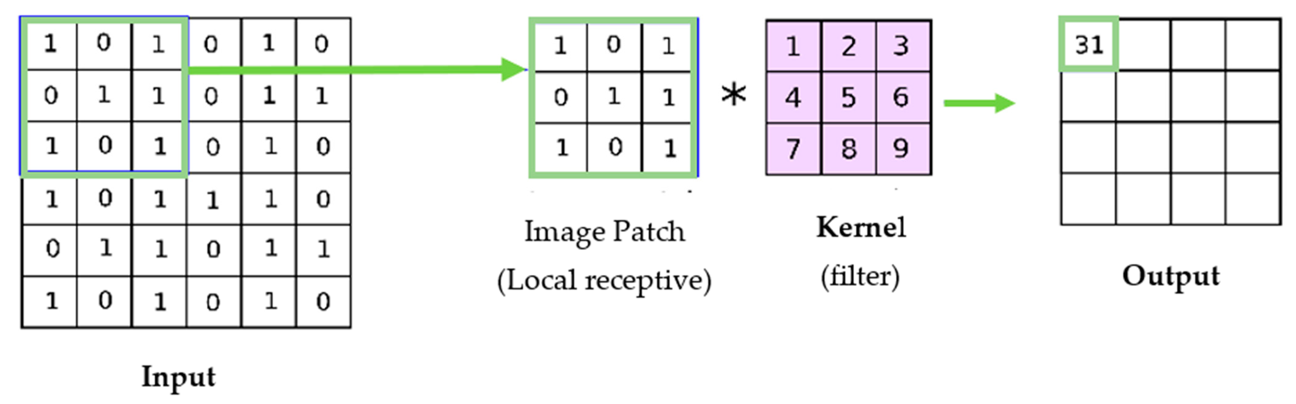
Figure 1. Convolutional process.
1.1.2. Pooling Layer
In CNN, the convolutional operation is applied to learned filters to the input image to summarize and show the presence of those features in the given. This is done in a systematic way to build its feature maps. The feature map is generated by the convolutional layer’s output. It has one limitation due to recording the exact location of features in the input. Therefore, in the input image, any small movement that happens to the position of a feature, such as re-cropping, rotation, etc., will cause changes in the feature map. A common solution to this problem can be achieved in the convolution layer using downsampling by altering the convolution stride over the image [8]. This is where the usage of the pooling layer begins. It is nothing but a common and robust approach to the same problem. In a short pooling layer downsample, the previous layers’ feature map and pooling operations aid in the creation of an invariant representation for small input translations [9]. Additionally, there are several functions used for specifying the pooling procedure; the most common functions are the following [10]:
- (a)
-
Average pooling: This is used when the average value is desired for each patch on the feature map.
- (b)
-
Maximum pooling: This is commonly known as Max-pooling, and is used when the maximum value is desired for each patch on the feature map [10]. Below Figure 2, illustrate the working of average and maximum pooling.
-
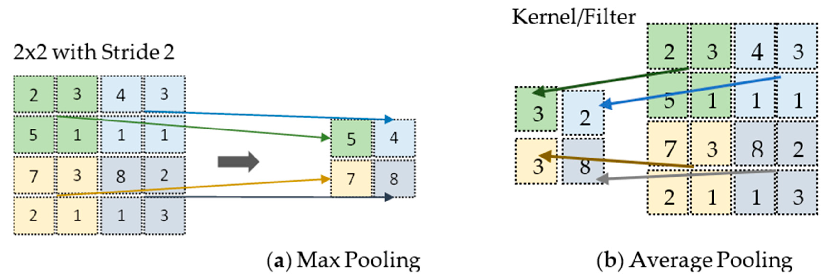 Figure 2. Two different pooling techniques were applied.
-
1.1.3. Fully Connected Layers
Immediately following the completion of feature extraction and consolidation by the convolutional and pooling layers, another layer comes in, which is known as the fully connected layer [11]. This component is connected to the final node of each network to flatten out the output of the previous layer. Finally, this layer returns the probability of class predictions by building non-linear feature combinations. There are various non-linear functions, such as activation functions, ReLU, and Softmax.
2. Important Parameters and Hyperparameters for Building Convolutional Neural Networks
The following are the important parameters with a high level of description.
-
Kernels: The kernel is nothing but a matrix that is used to traverse over the input images to perform a dot product to extract features [12]. By using the stride value, the kernel can move by columns of pixels based on the number assigned to the stride.
-
Biases: Before passing the output values through an activation function, the bias is used to adjust the scaled values. For example, in a neural network, the activation function receives an input ‘x’ which is multiplied by the ‘w’ weight. Therefore, adding a constant bias to the input will enable you to shift the activation function [13].
-
Padding: When a kernel is used with image processing, the image is altered each time a convolution is carried out on the input data. The image shrinks and thus this can be done only a certain number of times before the input image completely disappears [14]. As a result, some of the information contained in the image can be lost. The problem is that when the kernel moves across the image there is a significant impact on the pixels in the outskirts of the image, which are much smaller when compared to the center pixels of the image [15]. Therefore, a more accurate analysis of the image can be achieved by the use of padding, which is added to the image’s outer frame to provide more room for the filter to cover the image.
-
Stride: Stride is another so-called hyperparameter in the convolutional layer that specifies the pixel count the kernel shifts over the input image matrix. For instance, when two is set as the stride, then the filter or kernel moves two pixels at a time. When three is set as stride, then the filter moves three pixels at a time, and so on [16].
-
Dropout for regularization: This is a powerful yet simple regularization technique for deep learning models [17], and CNNs usually have the habit of overfitting. When there are a large number of nodes or neurons in a full-connected layer, it is more likely that co-adaptation occurs. Co-adaption simply means when many neurons in a single layer extract very similar or the same hidden features from the given input data. This usually happens when two different neurons’ connection weights are identical [18]. This technique works based on selecting neurons randomly and ignoring them during training; they will lose their contribution for further processes.
-
Learning Rate: The learning rate is a very important parameter in CNN which defines how swiftly a network updates its parameters during backpropagation [19]. Keeping the learning rate low makes the convergence smooth, but the learning process slows down. However, keeping the learning rate larger may speed up the process of learning, but may prevent convergence.
Activation Functions: Nonlinearity is introduced to models via activation functions, allowing deep-learning models to learn nonlinear prediction bounds. In artificial neural networks (ANNs), activation functions are used to transform an input signal into an output signal. This output signal is then used as input by the subsequent layer in the stack. The most common activations used in CNN are described below:
Sigmoid activation function: Because it is a non-linear function, it is the most often utilized activation function. The sigmoid function changes data in the 0 to 1 range and it is widely used for binary classification. It can be summed up as follows [20]:
Tanh activation function: It is a function known as the hyperbolic tangent. The Tanh function is comparable to the sigmoid function; however, it is symmetric concerning the origin [20]. This activation function is smoother, and it is a zero-centered function with a scale that goes from −1 to 1, therefore, the function’s output is given as [21]:
In contrast to the sigmoid function, the Tanh function became the favored function because it provides higher training performance for a model with multiple layers [22][23].
ReLU function: ReLU stands for the rectified linear unit; it is a non-linear function and very popular in ConvNets. Since all the neurons are not going to be activated at the same time, but rather a small number of neurons are activated at a time, the ReLU function is more efficient than others [20]. According to equation 1, the output of ReLU is the value that is greater than either zero or the value that was fed into the model. When the value of the input is negative, the value of the output is equal to 0. When the value of the input is positive, the output value will be equal to the value of the input [24].
An improved version of the ReLU activation function came up after ReLU, where instead of specifying the ReLU function’s value as zero for x (negative values), rather it is defined as an x having an extremely insignificant linear component. It can be mathematically stated as [20]:
Softmax activation function: For binary (0, 1) classification, the sigmoid function is used, but to deal with multiclass classification Softmax is used. The Softmax function returns a probability for each data point of all individual classes [20]. Therefore, in a deep neural network, when rwesearchers want to work with a multiclass classification problem, the output layer of the neural network will have an identical amount of network neurons that correspond to the number of target classes. The formula is stated as follows [25]:
Figure 3 represents the process for these connected layers.
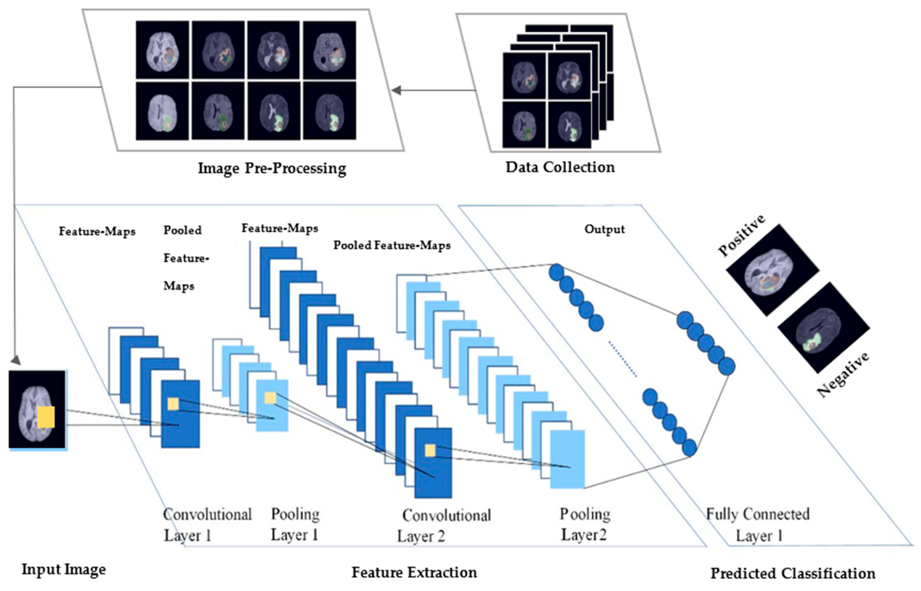
Figure 3. The diagram represents the medical image data collection. After collection, the images are preprocessed then given as input to the CNN model. There are a total of five layers: two conv-layers, two max-pooling layers.and an output layer called fully connected layer. The conv-weights in the first conv-layer are used in extracting feature maps from the input. Each pooled layer reduces the image size by half. Following the completion of each layer of pooling, the number of feature mappings and conv-weights are both increased by one. With the activation function, the last layer of the feature maps is fully connected to data nodes. Using a function, these nodes are then linked together to form a single value. This value was fitted to be the label defined in the training set and finally returned a value range of 0 and 1 [26].
3. ConvNets over Traditional Machine Learning
The process of machine learning involves the use of algorithms to analyze data, draw conclusions from that analysis, and make decisions based on those conclusions. In the case of DL, it uses multiple layers to create an ANN [27]. Each layer provides different information about the data which is fed to them. To perform classification work using machine learning techniques, several preprocessing steps, such as feature selection, [28], feature extraction [29], and classification are required [30]. Even the selection of features can have a significant impact on the efficiency gains achieved through various machine-learning strategies. DL techniques can perform automated feature sets for various tasks. Deep learning has simplified the improvement of object detection, image super-resolution, image classification, and image recognition fields [31].
Typical healthcare applications of classification tasks of images include Alzheimer’s disease (AD) classification using MRI [32], dermatological identification of skin conditions [33], breast cancer diagnosis using histopathological images [34], and diagnosis of eye diseases in the field of ophthalmology (such as diabetic retinopathy [35], corneal diseases [36], and glaucoma [37]). With advances in 2021, DL has become a key popular tool for the automatic detection of COVID-19 and classifying healthy and not-healthy individuals using X-rays and CT scan images [32].
3.1. The Problem with Traditional Neural Networks
The main significant distinction between the traditional ANNs and CNNs is the primary usage of ConvNets in the field of pattern recognition, in particular of medical images. This usage enables the developers to encode features of input images into the architecture and makes the convolutional neural network more beneficial for image-specific tasks, while also lowering the number of parameters needed to set up and build the model. Traditional neural networks are known as multilayer perceptrons (MLPs). MLPs have several limitations, particularly when it comes to the processing of images [38]. For each input, MLPs are going to use a single perceptron, which means if rwesearchers input an RGB image, each pixel is going to be multiplied by three since there are three channels in RGB. Therefore, here is where the problem arises; the number of weights to be used in each perceptron rapidly increases for large images, so it becomes unmanageable for the model. There are approximately 187,000 weights to train for a 250 × 250-pixel image with three channels. Hence, overfitting can happen, and training becomes difficult [39].
3.2. Feature Extraction
Feature extraction entails the process of obtaining a high level of patterns from raw pixel values to seize the uniqueness of the distinction between the various categories that are being used. The extraction of these features is carried out without the presence of any supervision (unsupervised manner). This indicates that the information that is extracted from the pixels of the image has nothing to do whatsoever with the classes of the image, and, in CNN, the convolution layer is the backbone of feature extraction [40]. This allows for the sharing of parameters. Following the extraction of the features [41], a classifier is then trained using the images and the labels that are associated with them, for example, logistic regression, random forests, decision trees, support vector machines, etc. This pipeline has a problem due to the fact that the feature extraction cannot be changed based on the classes and images. So, no matter what type of classification technique is used, the accuracy of the model is severely compromised as a result if the chosen feature does not give enough information to tell the categories apart [42]. Picking various feature extractors and clubbing them ingeniously to achieve better feature extraction has been a recurrent subject among state of the art studies. However, this necessitates an excessive number of heuristics and tedious manual work to adjust settings depending on the domain. The main philosophy behind deep learning is that there is no predetermined way to extract features (no hard-coding) from data [43]. The CNN learns to extract data by differentiating representations from the input images and to categorize them based on supervised data, all inside a single integrated system.
3.3. Parameter Sharing
With ConvNets, a large dataset like ImageNet can be used to train the whole network from scratch [44]. ImageNet is an ongoing project that has so far collected 14,197,122 images in 21,841 different categories. Sharing parameters cuts down on the total parameters in the network and shortens the training time required for the network [42].
References
- Wiesel, T.N. Receptive fields and functional architecture of monkey striate cortex. J. Physiol. 1968, 195, 215–243.
- Ghosh, A.; Sufian, A.; Sultana, F.; Chakrabarti, A.; De, D. Fundamental Concepts of Convolutional Neural Network. In Recent Trends and Advances in Artificial Intelligence and Internet of Things; Springer: Berlin/Heidelberg, Germany, 2019; pp. 519–567.
- Fukushima, K.; Miyake, S. Neocognitron learning by backpropagation. Syst. Comput. Jpn. 1995, 26, 19–28.
- Zhang, S.; Zhang, M.; Ma, S.; Wang, Q.; Qu, Y.; Sun, Z.; Yang, T. Research Progress of Deep Learning in the Diagnosis and Prevention of Stroke. BioMed Res. Int. 2021, 2021, 5213550.
- Jogin, M.; Mohana; Madhulika, M.S.; Divya, G.D.; Meghana, R.K.; Apoorva, S. Feature Extraction using Convolution Neural Networks (CNN) and Deep Learning. In Proceedings of the 2018 3rd IEEE International Conference on Recent Trends in Electronics, Information and Communication Technology, RTEICT 2018, Bangalore, India, 18–19 May 2018; pp. 2319–2323.
- Haq, A.U.; Li, J.P.; Khan, S.; Alshara, M.A.; Alotaibi, R.M.; Mawuli, C. DACBT: Deep learning approach for classification of brain tumors using MRI data in IoT healthcare environment. Sci. Rep. 2022, 12, 15331.
- Torres-Velazquez, M.; Chen, W.-J.; Li, X.; McMillan, A.B. Application and Construction of Deep Learning Networks in Medical Imaging. IEEE Trans. Radiat. Plasma Med. Sci. 2020, 5, 137–159.
- Brownlee, J. A Gentle Introduction to Pooling Layers for Convolutional Neural Networks. Mach. Learn. Mastery 2019, 22. Available online: https://machinelearningmastery.com/pooling-layers-for-convolutional-neural-networks/ (accessed on 5 December 2022).
- Naranjo-Torres, J.; Mora, M.; Hernández-García, R.; Barrientos, R.J.; Fredes, C.; Valenzuela, A. A Review of Convolutional Neural Network Applied to Fruit Image Processing. Appl. Sci. 2020, 10, 3443.
- Sun, M.; Song, Z.; Jiang, X.; Pan, J.; Pang, Y. Learning Pooling for Convolutional Neural Network. Neurocomputing 2017, 224, 96–104.
- Liu, T.; Fang, S.; Zhao, Y.; Wang, P.; Zhang, J. Implementation of Training Convolutional Neural Networks. arXiv 2015, arXiv:1506.01195, preprint.
- Mac, S.; Products, S.; Also, C. Convolutional Kernel Networks Julien. arXiv 2014, arXiv:1406.3332, preprint.
- Corvil. The Role of Bias in Neural Networks. 2018. Available online: https://www.pico.net/kb/the-role-of-bias-in-neural-networks/ (accessed on 16 March 2022).
- Skalski, P. Gentle Dive into Math Behind Convolutional Neural Networks. Data Sci. 2019. Available online: https://towardsdatascience.com/https-medium-com-piotr-skalski92-deep-dive-into-deep-networks-math-17660bc376ba (accessed on 20 February 2023).
- Hashemi, M. Enlarging smaller images before inputting into convolutional neural network: Zero-padding vs. interpolation. J. Big Data 2019, 6, 1–13.
- Prabhu. Understanding of Convolutional Neural Network (CNN)—Deep Learning. Medium. 2022. Available online: https://medium.com/@RaghavPrabhu/understanding-of-convolutional-neural-network-cnn-deep-learning-99760835f148 (accessed on 15 February 2023).
- Srivastava, N.; Hinton, G.; Krizhevsky, A.; Sutskever, I.; Salakhutdinov, R. Dropout: A Simple Way to Prevent Neural Networks from Overfitting. J. Mach. Learn. Res. 2014, 15, 1929–1958.
- Adrian, G. Dropout in Recurrent Neural Networks. 2018. Available online: https://adriangcoder.medium.com/a-review-of-dropout-as-applied-to-rnns-72e79ecd5b7b (accessed on 12 October 2022).
- Radhakrishnan, P. What are Hyperparameters? And How to tune the Hyperparameters in a Deep Neural Network? Data Sci. 2017. Available online: https://towardsdatascience.com/what-are-hyperparameters-and-how-to-tune-the-hyperparameters-in-a-deep-neural-network-d0604917584a (accessed on 20 February 2023).
- Sharma, S.; Sharma, S.; Anidhya, A. Understanding Activation Functions in Neural Networks. Int. J. Eng. Appl. Sci. Technol. 2020, 4, 310–316.
- Nwankpa, C.; Ijomah, W.; Gachagan, A.; Marshall, S. Activation Functions: Comparison of trends in Practice and Research for Deep Learning. arXiv 2018, arXiv:1811.03378. preprint.
- Neal, R.M. Connectionist learning of belief networks. Artif. Intell. 1992, 56, 71–113.
- DeepAI. ReLu Definition. In Deep AI Machine Learning Glossary; DeepAI; Available online: https://deepai.org/machine-learning-glossary-and-terms/relu (accessed on 22 February 2023).
- Agostinelli, F.; Hoffman, M.; Sadowski, P.; Baldi, P. Learning activation functions to improve deep neural networks. In Proceedings of the 3rd International Conference on Learning Representations, ICLR 2015—Workshop Track Proceedings, San Diego, CA, USA, 7–9 May 2015; pp. 1–9.
- Kim, M.; Yun, J.; Cho, Y.; Shin, K.; Jang, R.; Bae, H.-J.; Kim, N. Deep Learning in Medical Imaging. Neurospine 2019, 16, 657–668.
- IEEE. Engineering in Medicine and Biology Society. In Proceedings of the IECBES, IEEE-EMBS Conference on Biomedical Engineering and Science, Kuching, Malaysia, 3–6 December 2018.
- Khan, S. Business Intelligence Aspect for Emotions and Sentiments Analysis. In Proceedings of the 2022 First International Conference on Electrical, Electronics, Information and Communication Technologies (ICEEICT), Trichy, India, 16–18 February 2022; pp. 1–5.
- Khan, S.; AlSuwaidan, L. Agricultural monitoring system in video surveillance object detection using feature extraction and classification by deep learning techniques. Comput. Electr. Eng. 2022, 102, 108201.
- Boutahir, M.K.; Farhaoui, Y.; Azrour, M. Machine Learning and Deep Learning Applications for Solar Radiation Predictions Review: Morocco as a Case of Study. In Digital Economy, Business Analytics, and Big Data Analytics Applications; Springer: Berlin/Heidelberg, Germany, 2022; pp. 55–67.
- Alzubaidi, L.; Zhang, J.; Humaidi, A.J.; Al-Dujaili, A.; Duan, Y.; Al-Shamma, O.; Santamaría, J.; Fadhel, M.A.; Al-Amidie, M.; Farhan, L. Review of deep learning: Concepts, CNN architectures, challenges, applications, future directions. J. Big Data 2021, 8, 53.
- Jain, R.; Jain, N.; Aggarwal, A.; Hemanth, D.J. Convolutional neural network based Alzheimer’s disease classification from magnetic resonance brain images. Cogn. Syst. Res. 2019, 57, 147–159.
- Wu, H.; Yin, H.; Chen, H.; Sun, M.; Liu, X.; Yu, Y.; Tang, Y.; Long, H.; Zhang, B.; Zhang, J.; et al. A Deep Learning, Image Based Approach for Automated Diagnosis for Inflammatory Skin Diseases. Available online: https://www.ncbi.nlm.nih.gov/pmc/articles/PMC7290553 (accessed on 5 December 2022).
- Ting, D.S.W.; Cheung, C.Y.-L.; Lim, G.; Tan, G.S.W.; Quang, N.D.; Gan, A.; Hamzah, H.; Garcia-Franco, R.; Yeo, I.Y.S.; Lee, S.Y.; et al. Development and Validation of a Deep Learning System for Diabetic Retinopathy and Related Eye Diseases Using Retinal Images from Multiethnic Populations with Diabetes. JAMA 2017, 318, 2211–2223.
- IEEE. 2017 IEEE 19th International Conference on e-Health Networking, Applications and Services (Healthcom); IEEE: Piscataway, NJ, USA, 2017.
- Gu, H.; Guo, Y.; Gu, L.; Wei, A.; Xie, S.; Ye, Z.; Xu, J.; Zhou, X.; Lu, Y.; Liu, X.; et al. Deep Learning for Identifying Corneal Diseases from Ocular Surface Slit-Lamp Photographs. Available online: https://www.nature.com/articles/s41598-020-75027-3 (accessed on 5 December 2022).
- Bai, X.; Niwas, S.I.; Lin, W.; Ju, B.-F.; Kwoh, C.K.; Wang, L.; Sng, C.C.; Aquino, M.C.; Chew, P.T.K. Learning ECOC Code Matrix for Multiclass Classification with Application to Glaucoma Diagnosis. J. Med. Syst. 2016, 40, 78.
- Xin, M.; Wang, Y. Research on image classification model based on deep convolution neural network. EURASIP J. Image Video Process. 2019, 2019, 40.
- Brown, M.; An, P.E.; Harris, C.J.; Wang, H. How Biased is Your Multi-Layered Perceptron? World Congr. Neural Netw. 1993, 507–511. Available online: https://eprints.soton.ac.uk/250244/ (accessed on 22 February 2023).
- Haq, A.U.H.; Li, J.P.L.; Agbley, B.L.Y.; Khan, A.; Khan, I.; Uddin, M.I.; Khan, S. IIMFCBM: Intelligent Integrated Model for Feature Extraction and Classification of Brain Tumors Using MRI Clinical Imaging Data in IoT-Healthcare. IEEE J. Biomed. Health Inform. 2022, 26, 5004–5012.
- Guezzaz, A.; Benkirane, S.; Azrour, M.; Khurram, S. A Reliable Network Intrusion Detection Approach Using Decision Tree with Enhanced Data Quality. Secur. Commun. Networks 2021, 2021, 1230593.
- ResNet; AlexNet; VGGNet. Inception: Understanding Various Architectures of Convolutional Networks. 2022. Available online: https://cv-tricks.com/cnn/understand-resnet-alexnet-vgg-inception/ (accessed on 23 February 2023).
- Wang, P.; Fan, E.; Wang, P. Comparative analysis of image classification algorithms based on traditional machine learning and deep learning. Pattern Recognit. Lett. 2020, 141, 61–67.
- Suganyadevi, S.; Seethalakshmi, V.; Balasamy, K. A review on deep learning in medical image analysis. Int. J. Multimed. Inf. Retr. 2021, 11, 19–38.
- Shamshirband, S.; Fathi, M.; Dehzangi, A.; Chronopoulos, A.T.; Alinejad-Rokny, H. A review on deep learning approaches in healthcare systems: Taxonomies, challenges, and open issues. J. Biomed. Inform. 2020, 113, 103627.
More