Your browser does not fully support modern features. Please upgrade for a smoother experience.
Please note this is a comparison between Version 2 by Conner Chen and Version 1 by Srishti Gaur.
Land use land cover (LULC) modeling is considered as the best tool to comprehend and unravel the dynamics of future urban expansion.
- hybridization
- LULC modeling
- policy framework
1. LULC Modeling
With the advancement in data acquisition techniques (e.g., satellite imagery, citizen science-based approaches, and big-data platforms) and computational power, land use land cover (LULC) modeling practices have made substantial progress. Like other modeling techniques, the major phases associated with LULC modeling are calibration, simulation, validation, and prediction [1,11][1][2]. The data collection is the crucial pre-modeling step. Data can be obtained from satellite imagery, land surveys, and different online portals (e.g., census). The collected data are further used to develop the LULC maps using image classification techniques. Moreover, the data are also required for different explanatory variables responsible for the LULC changes. The explanatory variables are the drivers of LULC change ranging from bio-physical, proximity, demographic, socio-economic, economic, and institutional factors. The prominence of explanatory variables varies from region to region; however, the demographic factors (e.g., population growth) are the prominent factors in LULC changes [12][3].
The first stage of LULC models (i.e., model calibration) utilize the historical LULC information at different time intervals (say t1 and t2) and explanatory variables to estimate the amount of change to parameterize the model [6][4]. The simulation phase generates transition probability maps (TPMs) based on the potential explanatory variables [11][2]. TPMs, also called suitability or propensity maps, determine the potential location subject to LULC changes in the future [t3]. The third phase, model validation, estimates model accuracy in predicting the LULC changes. For this purpose, LULC prediction was performed for a time step (say t3) for which the measured LULC information was also available, and the accuracy of the model was estimated by comparing the predicted LULC with the measured LULC datasets [1]. The last phase of the LULC modeling predicts the future LULC by utilizing a well-calibrated/validated model. Figure 1 presents the schematic of the LULC modeling process. A significant limitation associated with the LULC modeling is that these models can accurately predict the LULC changes for a short time, varying from 2–3 decades. The reason behind this limitation is their dependency on historical patterns of change to predict the future LULC, which can perform reliable predictions for a short duration [13][5]. The following section discusses the details of different LULC models.
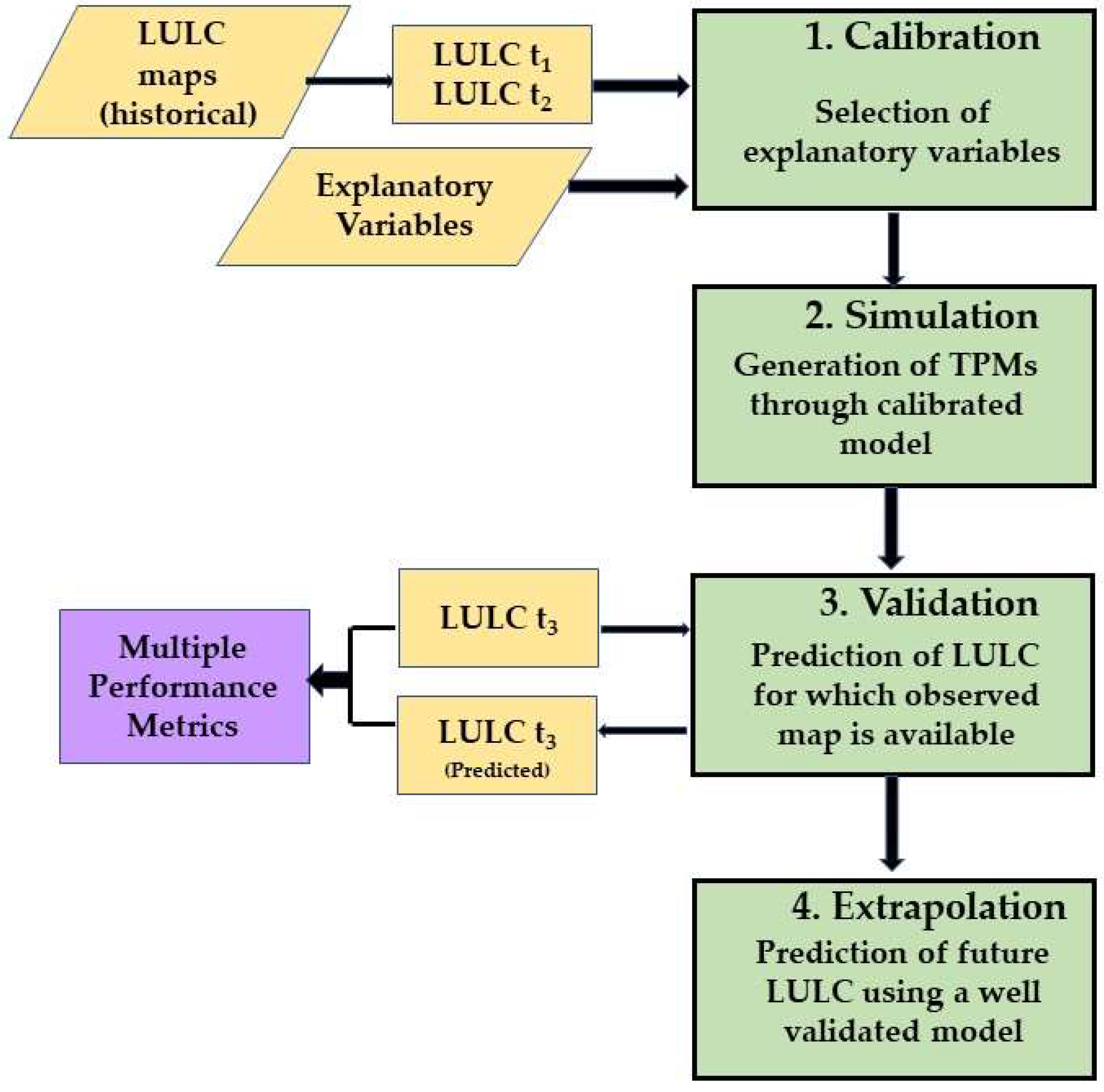
Figure 1.
Schematic of the LULC modeling processes.
A wide range of explanatory variables affects the LULC changes including bio-physical, proximity, socioeconomic, and economic variables. The bio-physical variables include the prevailing environmental conditions for LULC change, with a number of biotic and abiotic factors (i.e., soil, terrain, climate, lithology, vegetation, and topography) [1,14][1][6]. The proximity factors are based on the proximity concept, so the areas closer to the prevailing LULC class are more inclined to change in the other LULC class. The proximity factors include proximity to roads, rivers, cities, reservoirs (or waterbody), rail networks, and stream networks [13][5]. The other proximity factor associated with urban planning and management is distance to the city center, distance to shopping stores, and distance to schools. Socioeconomic factors include demographics, literacy rate, urbanization, industrialization, and regional gross domestic product (GDP). Demographic factors such as population growth are the prominent factors in LULC change [13,14][5][6]. Moreover, economic factors encompass a direct impact on decision-making (e.g., taxes, subsidies, demands, production and transportation costs, trade, capital flows and investments, technology, and credit access). Among the economic factors, taxes and subsidies are considered the major driving factor for LULC changes.
Accuracy estimation is a very important step for the validation of LULC models. Furthermore, the use of multiple performance metrics is recommended to ensure the credibility of the model. The Kappa-matrix is the most commonly used evaluation measure for LULC prediction, however, several researchers have criticized its use for accuracy assessment in remote sensing applications [15][7]. Relative operating characteristics are another important quantitative metric used to validate a LULC model. Moreover, Gaur et al. [1] used the chi-square goodness of fit test to evaluate the performance of the LULC model.
2. Statistical Models
Statistical models predict the LULC changes by establishing a mathematical relationship between the explanatory variables and LULC patterns [16][8]. The established relationship is utilized further to generate the TPMs. The popular statistical models used to estimate the quantity and patterns of LULC changes are regression-based models (e.g., linear regression and logistic regression, generalized additive models) and stochastic models (e.g., Markov chains). These models are often combined with other models such as cellular automata or genetic algorithms.
The significant advantage of these models lies in their ease of implementation and generalizability. However, these models do not perform well in cases where the explicit representation of human-based decision-making is required (e.g., farmers’ perception of agricultural intensification). In such cases, process-based models outperform statistical models. These models primarily deal with the simulation of the temporal analysis of change and lag behind the spatial analysis of changes [9]. Table 1 presents the details of the statistical models.
Table 1.
Details of the statistical models.
| Model | Underlying Assumptions | Example | Software |
|---|---|---|---|
| Statistical | Stationarity | Logistic regression | DYNAMICA/LCM model |
| Markov Models | |||
| Generalized linear modeling | |||
| Generalized additive modeling |
3. Cellular Automata (CA) Models
CA models utilize certain transition rules, neighborhood effects, and expert knowledge to analyze the spatial dynamics of change [16,17][8][10]. The spatial discretization units are pixels, cells, and parcels. CA models generate suitability maps instead of TPMs to estimate the spatial analysis of change [18][11]. These models simulate the LULC changes based on historical patterns and allocation based on the suitability of change and neighborhood interaction.
CA models apply both top–down and bottom–up approaches to simulate the LULC changes. Top–down determines the amount of LULC changes when the observations are available for the entire region of interest; however, the bottom–up approaches allocate the LULC change at the individual spatial unit. The major advantage of these models is that the decision-making process can be easily employed. These models can efficiently simulate the spatial analysis of change, however, lags in the temporal dynamic of change. Table 2 presents the details of the CA models.
Table 2.
Details of the cellular automata models.
| Model | Underlying Assumptions | Software |
|---|---|---|
| Cellular Models | Extrapolation of historical LULC patterns | CLUE-S |
| Allocation based on land suitability | CA | |
| Allocation by consideration of the state of neighborhood pixels | SLEUTH | |
| Dynamic CA-based model | Environment Explorer | |
| Model that simulates one-way transformation from one LULC class to another | GEOMOD |
4. Economic Model
Economic models simulate the LULC change as a market process [19][12]. Two types of economic models (i.e., sector-based and spatially disaggregated economic models) are widely used and differ by scale [20][13]. The sector-based models focus on the economic sector in the structural form to simulate the decisions on a more aggregated scale. Econometric models consider land as a fixed factor of production and illustrate demand and supply explicitly as contributors to market equilibria. The spatially disaggregated models simulate the decision at a smaller scale (e.g., field and neighborhood levels).
These models are advantageous in improving the trustworthiness of the economic processes leading to LULC changes [5][14]. However, the models also require assumptions of the market structures, functional forms, and economic processes. Table 3 presents the details of the economic models.
Table 3.
Details of the economic models.
| Model | Underlying Assumptions | Software |
|---|---|---|
| Economic models | Computable general equilibrium (CGE) |
FARM; GTAP; EPPA; IMAGE |
| Partial equilibrium (PE) | ASMGHG; IMPACT; GTM; AgLU; FASOM; GLOBIOM |
5. Agent-Based Models (ABMs)
ABMs consist of multi-agent systems and their interactions to simulate the complex LULC change processes [21][15]. Here, agents include farmers, laborers, landowners, policymakers, practitioners, professionals, and decision-makers who make decisions in LULC changes and processes (Figure 2) [22][16]. ABMs integrate the human decisions on LULC change and ponder the social interactions, adaptation, and development at multiple levels [23][17].
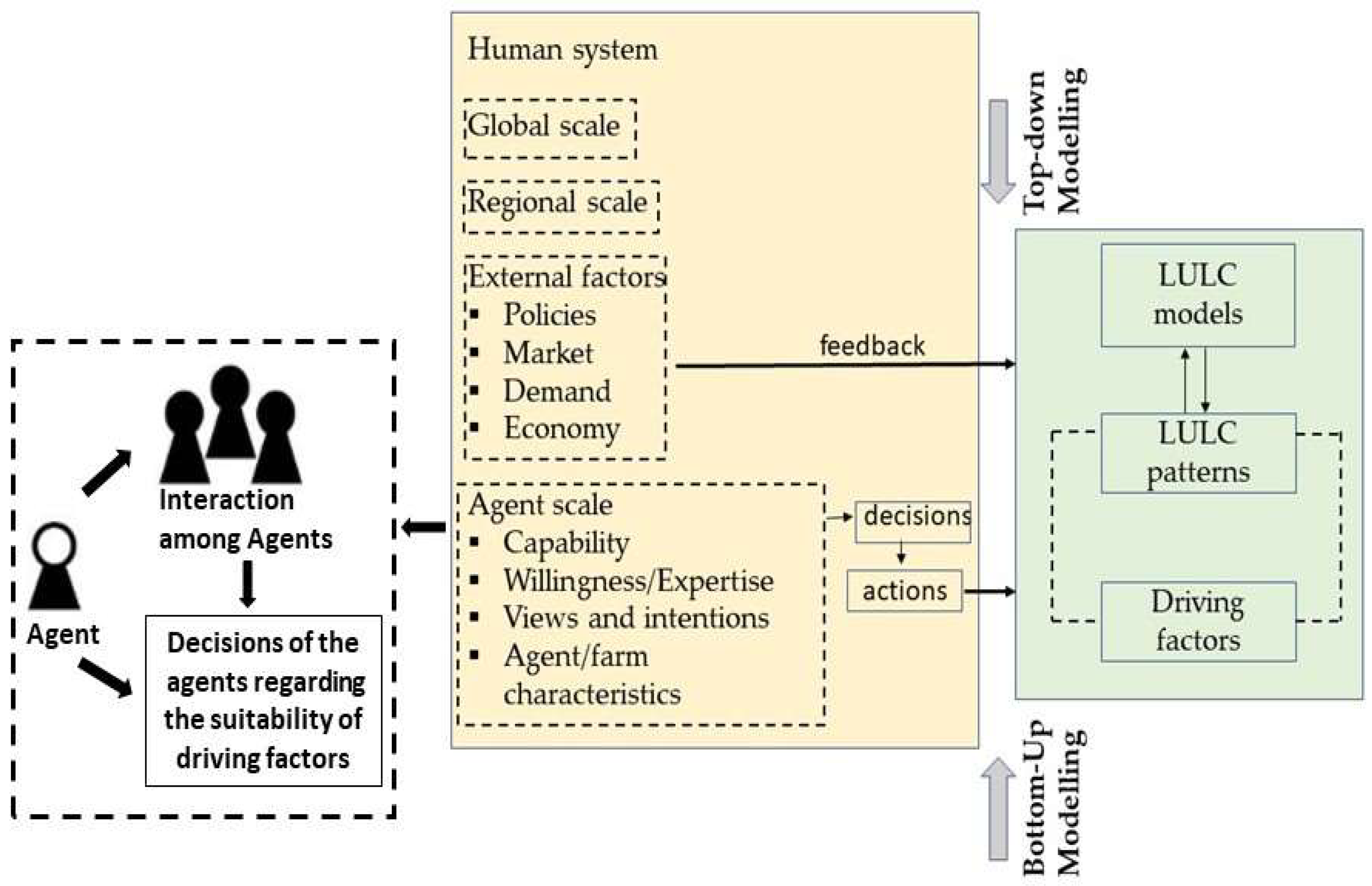
Figure 2.
A schematic of agent-based models.
ABMs facilitate the incorporation of expert elicitation and can communicate the model structure and functions to the stakeholders. However, these models lag in terms of generalization.
ABMs consist of independent decision-making entities (i.e., agents), an environment through which agents interact, and the rules that define the relationship between agents and their environment. With reference to a LUCC model, an agent may epitomize a land manager who combines individual knowledge and values, information on different driving factors (e.g., soil quality, climatic conditions, and topography), and an assessment of the land-management choices of neighbors (the spatial social environment) to calculate a land-use decision [24][18].
6. Hybrid Models
The idea behind the hybrid models is to combine the strength of individual models [10][19]. As each model has its advantages and disadvantages, hybrid models were invented to overcome the limitation of each model (e.g., the CA–Markov model is a hybrid of the CA and Markov models (statistical models)) [9,10][9][19]. CA models deal well with the spatial dynamics of change; however, it lags in simulating the temporal changes, so their integration with the Markov model could help overcome this issue.
The advantage of hybrid models is developing new methodologies that better represent reality. However, due to their complexity, these models are difficult to calibrate/validate.
7. Time Series Modeling for LULC Change
The time series modeling of LULC changes is another technique that is still in the evolution phase with the development of Earth observations. It utilizes multiple labeled time-series images for training to predict the LULC class labels of unlabeled time-series remote sensing images [25][20]. Remote sensing-based LULC monitoring approaches are classified into three categories (i.e., post-classification, pre-classification, and hybrid strategies) [26][21]. The post-classification approach deals with comparing the classified LULC maps with different time stamps and the overall accuracy determined by the product of individual map accuracies [27][22]. The pre-classification method has become feasible as satellite imagery has evolved with time, and has the potential to avoid the error accumulation issue that occurred in the post-classification method. The pre-classification method became viable as the satellite imagery archive grew over time [28[23][24],29], and has the capability to avoid the error accumulation issue that takes place in the post-classification technique. The LULC changes in the pre-classification technique are determined through the time-series analysis of vegetation indices. Moreover, the hybrid techniques utilize a combination of approaches to improve LULC monitoring (e.g., hybrid strategies such as the continuous change detection and classification algorithm [30][25]. LULC time-series monitoring has been widely used for the detection of global forest change [31][26].
References
- Gaur, S.; Mittal, A.; Bandyopadhyay, A.; Holman, I.; Singh, R. Spatio-Temporal Analysis of Land Use and Land Cover Change: A Systematic Model Inter-Comparison Driven by Integrated Modelling Techniques. Int. J. Remote Sens. 2020, 41, 9229–9255.
- Pontius, R.G.; Schneider, L.C. Land-cover Change Model Validation by an ROC Method for the Ipswich Watershed, Massachusetts, USA. Agric. Ecosyst. Environ. 2001, 85, 239–248.
- Kolb, M.; Mas, J.F.; Galicia, L. Evaluating Drivers of Land-Use Change and Transition Potential Models in a Complex Landscape in Southern Mexico. Int. J. Geogr. Inf. Sci. 2013, 27, 1804–1827.
- Mas, J.F.; Kolb, M.; Paegelow, M.; Camacho Olmedo, M.T.; Houet, T. Inductive pattern-based land use/cover change models: A comparison of four software packages. Environ. Model. Softw. 2014, 51, 94–111.
- Gaur, S.; Bandyopadhyay, A.; Singh, R. From Changing Environment to Changing Extremes: Exploring the Future Streamflow and Associated Uncertainties Through Integrated Modelling System. Water Resour. Manag. 2021, 35, 1889–1911.
- Gaur, S.; Krishna, C.T.; Bandyopadhyay, A.; Singh, R. Diagnosing the Combined Impact of Climate and Land Use Land Cover Changes on the Streamflow in a Mountainous Watershed. In Sustainability of Water Resources. Water Science and Technology; Yadav, B., Mohanty, M.P., Pandey, A., Singh, V.P., Singh, R.D., Eds.; Springer: Cham, Switzerland, 2022; Volume 116.
- Pontius, R.G.; Millones, M. Death to Kappa: Birth of Quantity Disagreement and Allocation Disagreement for Accuracy Assessment. Int. J. Remote Sens. 2011, 32, 4407–4429.
- Serneels, S.; Said, M.Y.; Lambin, E.F. Land Cover Changes around a Major East African Wildlife Reserve: The Mara Ecosystem (Kenya). Int. J. Remote Sens. 2001, 22, 3397–3420.
- Arsanjani, J.J.; Helbich, M.; Kainz, W.; Boloorani, A.D. Integration of Logistic Regression, Markov Chain and Cellular Automata Models to Simulate Urban Expansion. Int. J. Appl. Earth Obs. Geoinf. 2013, 21, 265–275.
- NRC. Advancing Land Change Modeling: Opportunities and Research Requirements; National Research Council: Washington, DC, USA, 2014.
- Lin, Y.P.; Chu, H.J.; Wu, C.F.; Verburg, P.H. Predictive ability of logistic regression, auto-logistic regression and neural network models in empirical land-use change modeling-a case study. Int. J. Geogr. Inf. Sci. 2011, 25, 65–87.
- Islam, K.M.; Rahman, F.; Jashimuddin, F. Modeling Land Use Change Using Cellular Automata and Artificial Neural Network: The Case of Chunati Wildlife Sanctuary, Bangladesh. Ecol. Indic. 2018, 88, 439–453.
- Xiaohua, T.; Yongjiu, F. A review of assessment methods for cellular automata models of land-use change and urban growth. Int. J. Geogr. Inf. Sci. 2020, 34, 866–898.
- Ren, Y.; Lü, Y.; Comber, A.; Fu, B.; Harris, P.; Wu, L. Spatially explicit simulation of land use/land cover changes: Current coverage and future prospects. Earth-Sci. Rev. 2019, 190, 398–415.
- Calvin, K.V.; Snyder, A.; Zhao, X.; Wise, M. Modeling land use and land cover change: Using a hindcast to estimate economic parameters in gcamland v2.0. Geosci. Model Dev. 2022, 15, 429–447.
- Lambin, E.F.; Geist, H. Land-Use and Land-Cover Change: Local Processes and Global Impacts; The IGBP Global Change Series; Springer: Berlin/Heidelberg Germany; New York, NY, USA, 2006.
- Evans, T.P.; Phanvilay, K.; Fox, J.; Vogler, J. An agent-based model of agricultural innovation, land-cover change and household inequality: The transition from swidden cultivation to rubber plantations in Laos PDR. J. Land Use Sci. 2011, 6, 151–173.
- Parker, D.C.; Manson, S.M.; Janssen, M.A.; Hoffmann, M.J.; Deadman, P. Multi-agent systems for the simulation of land-use and land-cover change: A review. Ann. Am. Assoc. Geogr. 2009, 93, 314–337.
- Poelmans, L.; Van Rompaey, A. Complexity and Performance of Urban Expansion Models. Comput. Environ. Urban Syst. 2010, 34, 17–27.
- Jining, Y.; Wang, L.; Song, W.; Chen, Y.; Chen, X.; Deng, Z. A time-series classification approach based on change detection for rapid land cover mapping. ISPRS J. Photogramm. Remote Sens. 2019, 158, 249–262.
- Reba, M.; Seto, K.C. A systematic review and assessment of algorithms to detect, characterize, and monitor urban land change. Remote Sens. Environ. 2020, 242, 111739.
- Colditz, R.R.; Acosta-Velázquez, J.; Díaz Gallegos, J.R.; Vázquez Lule, A.D.; Rodríguez-Zúñiga, M.T.; Maeda, P.; Cruz Lopez, M.I.; Ressl, R. Potential effects in multiresolution post-classification change detection. Int. J. Remote Sens. 2012, 33, 6426–6445.
- Coppin, P.; Jonckheere, I.; Nackaerts, K.; Muys, B.; Lambin, E. Review Article Digital change detection methods in ecosystem monitoring: A review. Int. J. Remote Sens. 2004, 25, 1565–1596.
- Zhu, Z. Change detection using landsat time series: A review of frequencies, preprocessing, algorithms, and applications. ISPRS J. Photogramm. Remote Sens. 2017, 130, 370–384.
- Zhu, Z.; Woodcock, C.E. Continuous change detection and classification of land cover using all available Landsat data. Remote Sens. Environ. 2014, 144, 152–171.
- Xu, L.; Herold, M.; Tsendbazar, N.E.; Masiliūnas, D.; Li, L.; Lesiv, M.; Fritz, S.; Verbesselt, J. Time series analysis for global land cover change monitoring: A comparison across sensors. Remote Sens. Environ. 2022, 271, 112905.
More