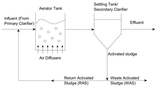
The activated sludge process (ASP) is the most widely used biological wastewater treatment system. Advances typical model that would simulate the ASP operation will have the following steps: a model objective, data collection, mathematical equations orin research have led to the adoption of Artificial Intelligence (AI), in particular, Nature-Inspired Algorithm (NIA) techniques such as Genetic Algorithms (GAs) and Particle Swarm Optimization (PSO) to optimize treatment systems. This has aided in reducing the complexity and computational time of ASP models for eachling.This paper covers the latest NIAs used in ASP as mentioned above, model calibration, and model validation. There are three main types of modellingnd discusses the advantages and limitations of each algorithm compared to more traditional algorithms that have been historically used foutilized over the ASP: deterministic or mechanistic modelling, stochastic modelling, and hybrid modelast few decades. Algorithms were assessed based on whether they looked at real/ideal treatment plant (WWTP) data (and efficiency) and whether they outperformed the traditional
algorithms combinin optimizing the two approaches.The most efficient models use hybrid models where stochastic modelling is used for the hard-to-define parameters and variablesASP. While conventional algorithms such as Genetic Algorithms (GAs), Particle Swarm Optimization (PSO), and Ant Colony Optimization (ACO) were found to be successfully employed in optimization techniques, newer algorithms such as Whale Optimization Algorithm (WOA), Bat Algorithm (BA), and IntensiveWeed Optimization Algorithm (IWO) achieved similar results in the treatment procesoptimization of the ASP, while also having certain unique advantages.
- wastewater treatment
- activated sludge process
- optimization
- nature inspired optimization
- nature inspired algorithms
- metaheuristic algorithms
1. Introduction

2. Modelling of Activated Sludge Process
A typical model that would simulate the ASP operation will have the following steps: a model objective, data collection, mathematical equations or models for each ASP as mentioned above, model calibration, and model validation [6]. Mathematical modelling has become an integral part of the design and operation of wastewater treatment processes, particularly the ASP. Simulations conducted with the models created have been a great source of value for ASP operators, designers, and even the wider scientific community. The main benefits of these models are the wide range of system functions and conditions that can be simulated and tested and solutions that can be found in a short time with low associated costs [7]. There are three main types of modelling that have been historically used for the ASP: deterministic or mechanistic modelling, stochastic modelling, and hybrid models combining the two approaches. The most efficient models use hybrid models where stochastic modelling is used for the hard-to-define parameters and variables in the treatment process. Deterministic modelling is used for the parts of the process that are both better understood and can be validated using the biological, physical, and chemical laws of the ASP [8]. Historically, deterministic models were the earliest type of work on activated sludge plants. Experimental data were taken and used to generate mathematical equations that depicted the relationship between variables in the various stages of the ASP. The most used mathematical model of the ASP was created by the International Association on Water Pollution Research and Control (IAWPRC) Task Group [9]—the Activated Sludge Model No. 1 (ASM1). Even though it was developed in 1987, researchers still widely use it for their work, albeit with modified versions. The main processes involved in the traditional ASM1 model were the microorganisms’ growth, maintenance, and decay. Nitrification and denitrification were also included in some models along the way. It was accepted that this simplified approach has some demerits due to considering only these few processes and components [8]. Over the years, many modifications have been made to the traditional model approach. For example, Eckhoff et al. [10] used COD instead of BOD as a parameter to calculate the inert fraction of the substrate. Models based on COD are generally preferred over BOD in academic/research models because they are better at conserving the mass oxygen balance. However, BOD models are used to better characterize influent wastewater [11]. There are a few drawbacks to the ASM1 model. The International Water Association (IWA) has only given reference values for the dynamic or stoichiometric parameters of the model and its application to a real-life WWTP (real/ideal treatment plant); the parameters will have to be corrected [12]. Different calibration data sets can produce the same results. Some variables used cannot be measured in the real-time process, making it hard to verify the model. Certain factors are not considered, such as the dependency of temperature and pH on the constants used. Calibration and model verification can be difficult and highly sensitive—sometimes, extensive lab equipment is required. Phosphorous removal was also not considered in this model, which created issues in practical application [13]. In 1995, a modified version of the ASM1 called the Activated Sludge Model No. 2 (ASM2) was developed, which included phosphorous removal in addition to carbonaceous and nitrogenous material. However, phosphorous removal is complex, thereby complicating the calibration and verification of the ASM2 model. The ASM1 and ASM2 were further improved by creating two models, Activated Sludge Model No. 2d (ASM2d) and Activated Sludge Model No. 3 (ASM3). ASM2d builds upon ASM2 by adding denitrifying activity of Polysulphate Accumulating Organisms that show better relation between phosphorous and nitrate. ASM3 was developed similar to ASM1 but considering the effect of storage polymers in heterotrophic activated sludge conversion [14]. To summarize, ASM1 can be used to simulate both carbon removal and denitrification, ASM2 simulates phosphorous removal in addition to decarbonization and denitrification, ASM2d further improved the relationship between phosphorous and nitrate in ASM2, and ASM3 improved upon ASM1 adding the effect of storage polymers. All the ASM models are mechanistic models where differential equations are used to describe and restore the dynamic changes in the wastewater treatment system. The models ASM1 and ASM2, ASM2d use the theoretical basis of death–regeneration and maintenance, whereas ASM3 utilizes the theoretical basis of endogenous microbial respiration [13]. Due to the many processes, variables, and parameters involved, activated sludge models are often validated and calibrated by trial and error with no standard procedure [8][15][8,15]. For example, Siegrist and Tschui [16] created several models with different sets of parameters for partial and sequential calibration. Calibration for COD removal was undertaken by considering the oxygen consumption rate when other parameters were held constant. The model was validated by comparing it with full-scale treatment plant data, where an example would be [17]. They created a dynamic model for carbon and nitrogen removal and validated it with data obtained from 10 days of monitoring Norwich Sewage Works in England. Côté et al. [18] used a hybrid model, which improved upon previous work by using a neural network to predict and reduce error in mechanistic model variables such as effluent suspended solids, effluent COD, and volatile solids in return sludge, etc. The mechanistic model was validated with data from Norwich Sewage Works.2.1. Artificial Intelligence Used in Modelling of WWTP
The traditional mechanistic models, such as ASM1, have reached a limit when considering the complexity and accuracy of application to the ASP, with some of the issues mentioned in Section 2. Thus, Artificial Intelligence can be used as a modelling tool to minimize the complexities and reduce computing time [19]. There are several different types of AI modelling tools adapted for different fields and functions. Of these are feedforward Artificial Neural Networks (ANNs); radial basis functions (RBFs); recurrent neural networks (RNNs); multilayer perceptron (MLP) using backpropagation learning; hybrid models such as adaptive neuro-fuzzy inference (ANFIS). More recently, deep neural networks (DNNs) contain multiple hidden layers and require significant computational power [20][21][20,21]. The traditional ANN has a few limitations such as poor generalization due to incorrectly chosen network structure, hard-to-interpret system information stored in neuron weights, and a large amount of data required for accuracy. ANFIS tends to overcome a few of these limitations [21]. Additionally, Feedforward Artificial Neural Networks (FANNs)—MLPs and RBFs—are commonly used in wastewater treatment operations. MLPs have been found to be better than regression models for wastewater treatment [8], whilst RBFs are useful because they can easily predict system behavior from past observations [22]. DNNs vary from typical feedforward neural networks (ANNs) because DNNs contain more neurons, complexity in connecting layers, more computing power required to train the network due to having more neurons/connections, and automatic feature extraction [22]. Some of these tools, along with applications in wastewater treatment, particularly the ASP, are discussed below.2.2. Artificial Neural Network (ANN)
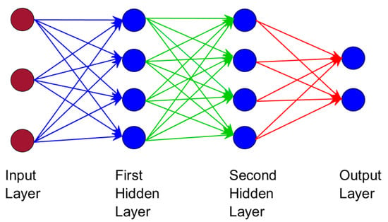
ANN is designed as a simplified version of the human brain, where inputted neurons generate output signals. The general structure of a neural network is shown in Figure 2, where there are layers of interconnected neurons. There are several layers: the input layer, where inputs are given as weights to input neurons; the output layer, where output neurons do processing based on the input using an activation function and generate output; and single/multiple hidden layers, where intermediary neurons process the weighted sums of the inputs. Sometimes, output neurons can also be connected to each other and not just to the previous inputs, but this is complex and uncommon [20][23][20,23].
