Your browser does not fully support modern features. Please upgrade for a smoother experience.
Please note this is a comparison between Version 1 by Mohsen Eslami Nazari and Version 2 by Dean Liu.
Oceans cover over 70% of the Earth’s surface and provide numerous services to humans and the environment. Therefore, it is crucial to monitor these valuable assets using advanced technologies. In this regard, Remote Sensing (RS) provides a great opportunity to study different oceanographic parameters using archived consistent multitemporal datasets in a cost-efficient approach. Various types of RS techniques have been developed and utilized for different oceanographic applications.
- remote sensing
- ocean
- ocean wind
- ocean current
1. Introduction
Oceans cover more than 70% of the Earth’s surface and provide countless benefits. For example, the oceans produce over 50% of the world’s oxygen and store carbon dioxide. Moreover, the oceans transport heat from the equator to the poles and regulate climate patterns. Additionally, oceans play a key role in transportation, food provision, and economic growth. Oceans are also important for recreational activities [1][2][3][1,2,3]. Considering the importance of ocean environments, it is important to protect them using advanced technologies. To this end, datasets collected by in situ, shipborne, airborne, and spaceborne systems are being utilized.
Although in situ measurements provide the most accurate datasets for ocean studies, they have several limitations. For example, they are point-based observations and cover small areas. Moreover, deployment and maintenance of in situ platforms (e.g., buoys) are expensive and labor-intensive [4]. Shipborne approaches also have their own disadvantages. For instance, they can only measure Ocean Surface Wind (OSW, see Table A1 for the list of acronyms) along specific tracks, and the vastness and remoteness of ocean environments hinder surveillance of human activities because authorities cannot frequently provide effective vessel control [5]. On the other hand, ocean mapping and monitoring using airborne and spaceborne Remote Sensing (RS) systems are of significant interest due to the large coverage, a wide range of temporal and spatial resolutions, as well as low cost of the corresponding datasets [6][7][8][6,7,8]. TheOur understanding of ocean environments, including marine animals, oceanic biogeochemical processes, and the relationship between oceans and climate changes, has considerably improved due to the availability of global, repetitive, and consistent archived satellite observations. It should be noted that although RS provides a great opportunity for ocean studies, it does not obviate the necessity of in situ measurements, and they usually play a supporting role to each other in different oceanographic applications.
Different methods have been so far developed to derive oceanographic parameters from RS datasets. These methods can be generally divided into three groups of statistical, physical, and Machine Learning (ML) models. Statistical algorithms are mainly based on the correlation relationships between in situ measurements of oceanographic parameters and the information collected by RS systems. These models are usually easy to develop and provide fairly reasonable accuracies. However, they require in situ data, which are sometimes not available over remote ocean areas. These models also need to be optimized for different study areas. Physical models (e.g., Radiative Transfer (RT)) are based on the physical laws of the RS systems. Although these models usually provide better results than statistical models, they require many inputs that are usually not available. Recently, ML algorithms, either traditional (e.g., Random Forest (RF) and Support Vector Machine (SVM)) or more advanced models (e.g., Convolutional Neural Network (CNN)), have been frequently utilized for various oceanographic applications. Generally, like many other applications of RS, Deep Learning (DL) methods provide higher accuracies compared to statistical, physical, and traditional ML algorithms [9][10][11][9,10,11]. However, it should be noted that DL methods require a very large number of training data and are computationally expensive [12]. Consequently, it is sometimes more reasonable to utilize other, less-costly ML algorithms [13][14][13,14].
3. RS Applications in Ocean
As discussed in the Introduction, six oceanographic applications of RS are explained in Part 1 of this review paper. These applications, along with the RS systems which can be used to study them, are illustrated in Figure 1. More detailed discussions are also provided in the following six subsections.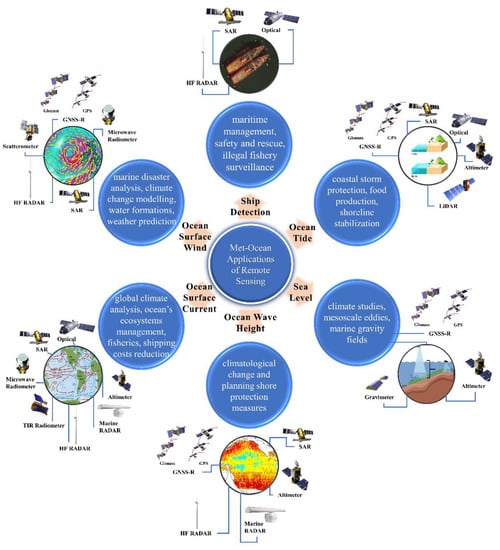
Figure 1. Overview of the met-ocean applications of RS which are discussed.
Overview of the met-ocean applications of RS which are discussed in this review paper.
3.1. Ocean Surface Wind (OSW)
OSW is an essential parameter for various applications, such as marine disaster monitoring, climate change modeling, water mass formations, and Numerical Weather Prediction (NWP) [15][16][17][18][76,77,78,79]. Considering the limitations of the traditional methods for OSW estimation (e.g., anemometers and buoys) [15][19][76,80], RS observations have emerged as cost-effective techniques [20][81]. Remotely sensed OSW information mainly relies on the relationship between the OSW and the sea surface roughness, which represents emissive and reflective properties of the ocean surface [18][79]. Five RS systems have been frequently applied to measure OSW: microwave radiometer, GNSS-R, SAR, scatterometer, and HF radar. The advantages and disadvantages of each system, summarized in Table 1, are discussed in more detail in the following subsections.Table 1. Different RS systems for OSW estimation along with their advantages and disadvantages.
| RS System (Passive/Active) | RS System (Type) | Advantage | Disadvantage |
|---|---|---|---|
| Passive | Microwave radiometer | Appropriate efficiency in high wind speeds, large-scale coverage | Low accuracy for OSW direction estimation in low wind speeds, coarse spatial resolution |
| GNSS-R | Higher spatial and temporal resolution, less sensitivity atmospheric attenuation, low-cost, low weight, low power needs for receivers, unique sensing geometry | Inadequate number of satellites, need more investigation and validation | |
| Active | SAR | High spatial resolution, applicable at both low and high wind speeds | Speckle noise issue, challenging preprocessing steps |
| Scatterometer | Good efficiency in low wind speeds, global coverage | Coarse spatial resolution, saturated signal in high wind speeds, rain contamination | |
| HF radar | Reasonable accuracy at different wind speeds, large-scale coverage | Availability of OSW data only at specific coastal locations where the HF radar has been installed |
3.2. Ocean Surface Current (OSC)
. Ocean Surface Current (OSC)
OSC is the continuous and directional movements of the mass of the seawater, transferring nutrients, energy, heat, pollutants, and chemical substances around the world [21][22][112,113]. Ocean currents affect the global climate, the ocean’s ecosystems, and fishing productivity. More importantly, they play a key role in reducing shipping costs, fuel consumption, as well as developing policies for preventing natural disasters [21][23][112,114]. OSC can originate from a wide range of factors, such as wind, Coriolis effect, water density variation, Ocean Tide (OT), as well as SST and OS differences [21][22][24][25][112,113,115,116]. The seafloor and shoreline topography can also affect OSC and hinder or boost the mixing and passageway of water from different areas [26][117]. Ocean currents can be generally divided into five categories: (1) geostrophic ocean current, which is balanced under pressure gradient force by the Coriolis effect; (2) tidal ocean current, which is created by the gravitational force of the moon, sun, and Earth; (3) wind-driven Ekman ocean current, which is created by the steady ocean wind; (4) wave-induced Stokes drift, which is characterized by the difference between the average Lagrangian flow velocity of a fluid parcel and the average Eulerian flow velocity of the fluid at a fixed position; and (5) small-scale ocean current, which is created by the small features such as eddies, fronts, and filaments [27][118]. Ocean currents are also separated into two groups based on their temperature: warm and cold ocean currents (see Figure 13) [3]. For instance, the Gulf stream, Kuroshio, and the Agulhas are warm currents that transport heat from the tropics poleward and significantly affect the global climate [21][28][29][112,119,120]. The Humboldt, Benguela, and California are cold currents that preserve highly upwelling waters and carry cold water toward the equator [21][29][112,120]. For example, the Labrador Current has a cooling effect with a low OS and is known for transporting icebergs from Greenland’s glaciers into shipping lanes in the North Atlantic [29][30][120,121].
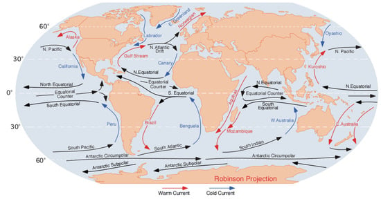
Figure 13. The global ocean currents, including warm currents (red line), cold currents (blue line), and neutral current (black line) adopted from https://commons.wikimedia.org/wiki/File:Corrientes-oceanicas.png (accessed on 8 October 2022).
Ocean currents can also be categorized into two groups according to their depth: surface and deep (subsurface) [21][27][31][112,118,122]. The surface currents are horizontal water streams that occur on local to global scales, and their effects are primarily restricted to the top 400 m of ocean water [21][32][112,123]. Along the coasts and offshore regions, there are local surface currents, which are typically small and short-lived (e.g., hourly/seasonal), generated by OT, waves, buoyant river plumes, and local-scale winds [21][32][112,123]. These currents control the local flooding, algal bloom, marine pollution, sediment transport, and ship navigation [21][32][112,123]. The global surface currents (e.g., the Gulf Stream) are typically controlled by dominant global winds (e.g., trade winds and the westerlies) together with Coriolis force and the restriction of flow by continental deflections [21][23][32][112,114,123]. These currents travel over long distances in the same direction as the wind and at a speed of approximately 3 to 4% of winds’ speed [21][32][112,123]. However, the Coriolis force deflects these currents from the equator to the right direction in the Northern Hemisphere and the left in the Southern Hemisphere, which creates the clockwise and counterclockwise circular patterns or gyres, respectively [21][23][24][32][33][112,114,115,123,124]. In contrast, the deep ocean currents are vertical streams under the influence of the thermohaline circulation generated by water density differences and depend on temperature and OS [21][34][112,125]. Deep ocean currents are formed with upwelling and downwelling directions below 400 m of the surface water [35][126].
Depending on the scale of the ocean currents, they are measured by different methods. Figure 24 illustrates various in situ and RS methods for ocean current estimation. It should be noted that the focus of this section is on the OSC using offshore, shipborne, and spaceborne platforms. Table 2 also summarizes these systems along with their advantages and limitations for OSC studies. More details about the applications of each system are also provided in the following subsections.
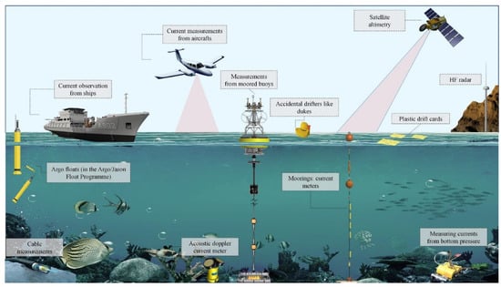
Figure 24.
Different methods for ocean current estimation.
Table 2.
Different RS systems for OSC estimation along with their advantages and limitations.
| RS System (Passive/Active) | RS System (Type) | Advantage | Disadvantage |
|---|---|---|---|
| Passive | Optical | Provides high spatial resolution images for retrieving and characterizing spatiotemporal OSC | Calibrating issues due to defining several input parameters, limited by cloud cover, requires a reliable operational procedure for feature tracking, not suitable for nighttime |
| TIR radiometers |
Mesoscale OSC fields retrieval based on the feature tracking at high temporal rates | Limited by cloud cover, edge-of-scan distortions, hard for features to evolve due to degradation of their surface signature | |
| Microwave radiometers | Can measure under clouds and in all weather conditions except for rain, OSC estimation at a global scale | Coarse resolution, limited to regions with sun-glitter, rain, or proximity to land | |
| Active | SAR | Not limited by cloud cover or daytime, contains physical properties, high spatial resolution, different data acquisition modes are available, ability to detect small leads, penetration capability | Difficult data interpretation, speckle noise, different ice types might have similar scattering behavior, similarity of wind roughened water and ice |
| Altimeter | Almost daily global coverage, accurate topography for SI thickness measurement, ability to map small leads | Error due to the roughened sea surface, no physical characteristics | |
| HF radar | Suitable for global-scale studies | Limited data availability, not frequent observations | |
| Marine radar | Not limited by cloud cover and daytime, long-time data archive | Unable to provide images, signal loss in propagation into dense ice, unable to detect SI presence constantly |
3.3. Ocean Wave Height (OWH)
. Ocean Wave Height (OWH)
Wind blowing over the ocean surface creates ocean waves with a different range of heights depending on the wind speed, wind duration, and distance. The resulting waves can travel for hundreds or even thousands of kilometers and form swell waves of various heights. Although waves are generally caused by wind, catastrophic waves (e.g., landslide surges, tsunamis, and storm surges) [36][151] and internal waves (e.g., subsurface waves at the boundary between two water layers) [37][152] can also generate ocean waves. OWH information is a critical parameter for coastal construction, ship navigation, and human activities in the oceans [38][153].
The datasets collected by different RS systems, such as GNSS-R, SAR, altimeter, and marine radar, have been utilized for OWH estimation. In this regard, various models have been applied to retrieve OWH from these datasets [39][154]. For example, due to the complexity of physical models (e.g., RT models), empirical and semiempirical models have also been developed to estimate OWH [40][155]. The simplicity of empirical and semiempirical models has also led to the development of ML algorithms [41][156]. In this regard, DL algorithms, as the most advanced ML models, have received more attention due to their promising performance. For example, Shao et al. [42][157] proposed a hybrid statistical and a DL model in South China to predict several ocean surface variables, including OWH. In Liu et al. [43][158], a short-term memory deep network was also proposed to consider the time domain data in OWH estimation. Table 3 summarizes the advantages and disadvantages of each of these RS systems. In the following subsections, the studies that have been conducted to measure OWH based on various RS systems are discussed in more detail.
 Conventionally, SL estimation was based on coastal monitoring stations, tide gauges, buoys, and ship surveys [51][212]. However, the high cost and sparse observations of these approaches make them inappropriate for SL measurements in most cases. Moreover, in situ measurements contain significant interannual and decadal effects and do not perfectly manifest the SL change [52][213]. However, with the advancement of RS technology, satellites provide valuable datasets to study SL at different local to global scales. In addition to studies that only focused on SL measurements using RS systems, many studies related SL observations to different environmental variables. Through these analyses, it was widely argued that the main contributors to SL rise are thermal expansion of seawater [53][214], Antarctic and Greenland ice sheet melting [54][215], and land-water storage change due to the groundwater depletion [55][216]. Consequently, SL rise has many environmental and economic impacts, including reef island destabilization [56][217], wave resource alteration [57][218], coastal erosion [58][219], saltwater intrusion into aquifers [59][220], sea turtle nesting threatening [60][221], lowland and delta vulnerability [61][222], coastal flooding [62][223], seaport infrastructure susceptibility [63][224], wetland inundation and displacement [64][225], island and offshore baseline loss [65][226], tidal dynamics [66][227], and length-of-day changes [67][228].
Among different RS systems, GNSS-R, altimeters, and gravimeters have been widely employed for SL studies [68][69][70][71][72][229,230,231,232,233]. The advantages and disadvantages of these systems applied for SL mapping are provided in Table 4. The following subsections discuss the applications of each system.
Conventionally, SL estimation was based on coastal monitoring stations, tide gauges, buoys, and ship surveys [51][212]. However, the high cost and sparse observations of these approaches make them inappropriate for SL measurements in most cases. Moreover, in situ measurements contain significant interannual and decadal effects and do not perfectly manifest the SL change [52][213]. However, with the advancement of RS technology, satellites provide valuable datasets to study SL at different local to global scales. In addition to studies that only focused on SL measurements using RS systems, many studies related SL observations to different environmental variables. Through these analyses, it was widely argued that the main contributors to SL rise are thermal expansion of seawater [53][214], Antarctic and Greenland ice sheet melting [54][215], and land-water storage change due to the groundwater depletion [55][216]. Consequently, SL rise has many environmental and economic impacts, including reef island destabilization [56][217], wave resource alteration [57][218], coastal erosion [58][219], saltwater intrusion into aquifers [59][220], sea turtle nesting threatening [60][221], lowland and delta vulnerability [61][222], coastal flooding [62][223], seaport infrastructure susceptibility [63][224], wetland inundation and displacement [64][225], island and offshore baseline loss [65][226], tidal dynamics [66][227], and length-of-day changes [67][228].
Among different RS systems, GNSS-R, altimeters, and gravimeters have been widely employed for SL studies [68][69][70][71][72][229,230,231,232,233]. The advantages and disadvantages of these systems applied for SL mapping are provided in Table 4. The following subsections discuss the applications of each system.
 A tidal channel is a type of stream or a waterway that occurs during the ebb tide and flood tide in the tidal flats [83][265]. Tidal channel networks are crucial aspects of the neighboring ocean and estuaries. In addition to the control of the tidal basin hydrodynamics, tidal channels connect intertidal flats to the salt marshes, which play an important role in tidal propagation [84][266]. Due to various morphological characteristics from terrestrial river networks, conventional river system algorithms cannot be implemented on tidal channels. Thus, RS techniques have been effectively utilized to obtain the spatial distribution of tidal channels [84][266].
The periodic movement of water created by the out-of-phase OT, the local weather patterns (radiational tides), and ocean characteristics (internal tides) is defined as tidal currents [85][267]. Periodic tidal currents play an important role in the strait (a narrow waterway joining two larger water bodies) [85][267]. Tidal currents’ power intensifies when flowing through the narrow and shallow channels in the islands or over the shallow ridges, although they are weak in most parts of the strait [86][268]. Furthermore, tidal current power is renewable and predictable energy [87][269], mostly occurring at narrow tidal channels. Tidal current generators not only cause fewer environmental concerns than barrages, but can also be installed incrementally to meet the increase in demand over time [88][270]. Therefore, mapping the tidal energy density is crucial to consider the economic possibility, while tidal currents vary regionally. In this regard, a higher level of measurements, including spring and neap tidal cycles and higher temporal and spatial measurements, are required [87][269].
OTL displacements are the elastic response of the Earth to the redistribution of water mass from OT, which can cause deformation gradients of several millimeters to centimeters near coastal regions [89][271]. One of the most productive inland and coastal ecosystems is tidal wetlands. Tidal wetlands are important for trapping sediment and pollution, recreational purposes, and flood control. They are also natural barriers against saltwater intrusion into freshwater aquifers [90][91][272,273]. The tidal regime, relative SL rise, land cover change, and sedimentation are driving factors influencing tidal wetlands [92][274]. Tides increase rates of relative SL rise, resulting in brackish water and a shift to becoming nontidal wetlands in freshwater tidal areas. So far, different RS systems have been successfully employed for OT studies. Table 5 summarizes the advantages and limitations of the RS systems that have been frequently used for OT measurement.
A tidal channel is a type of stream or a waterway that occurs during the ebb tide and flood tide in the tidal flats [83][265]. Tidal channel networks are crucial aspects of the neighboring ocean and estuaries. In addition to the control of the tidal basin hydrodynamics, tidal channels connect intertidal flats to the salt marshes, which play an important role in tidal propagation [84][266]. Due to various morphological characteristics from terrestrial river networks, conventional river system algorithms cannot be implemented on tidal channels. Thus, RS techniques have been effectively utilized to obtain the spatial distribution of tidal channels [84][266].
The periodic movement of water created by the out-of-phase OT, the local weather patterns (radiational tides), and ocean characteristics (internal tides) is defined as tidal currents [85][267]. Periodic tidal currents play an important role in the strait (a narrow waterway joining two larger water bodies) [85][267]. Tidal currents’ power intensifies when flowing through the narrow and shallow channels in the islands or over the shallow ridges, although they are weak in most parts of the strait [86][268]. Furthermore, tidal current power is renewable and predictable energy [87][269], mostly occurring at narrow tidal channels. Tidal current generators not only cause fewer environmental concerns than barrages, but can also be installed incrementally to meet the increase in demand over time [88][270]. Therefore, mapping the tidal energy density is crucial to consider the economic possibility, while tidal currents vary regionally. In this regard, a higher level of measurements, including spring and neap tidal cycles and higher temporal and spatial measurements, are required [87][269].
OTL displacements are the elastic response of the Earth to the redistribution of water mass from OT, which can cause deformation gradients of several millimeters to centimeters near coastal regions [89][271]. One of the most productive inland and coastal ecosystems is tidal wetlands. Tidal wetlands are important for trapping sediment and pollution, recreational purposes, and flood control. They are also natural barriers against saltwater intrusion into freshwater aquifers [90][91][272,273]. The tidal regime, relative SL rise, land cover change, and sedimentation are driving factors influencing tidal wetlands [92][274]. Tides increase rates of relative SL rise, resulting in brackish water and a shift to becoming nontidal wetlands in freshwater tidal areas. So far, different RS systems have been successfully employed for OT studies. Table 5 summarizes the advantages and limitations of the RS systems that have been frequently used for OT measurement.
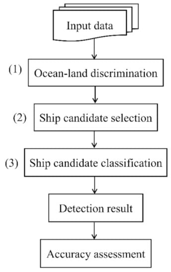
SD methods using spaceborne RS (i.e., optical and SAR) datasets generally have three main steps (see Figure 59): (1) ocean–land segmentation, (2) ship candidate extraction, and (3) classification of ship candidates [99][100][101][319,320,321]. Since the objective of the corresponding studies is to detect ships in oceans, the first step is separating ocean and land regions. This is usually performed using GIS layers of coastlines. However, with the end-to-end DL SD methods, this step is not necessary anymore. Most of the SD research studies have focused on the second and third steps by developing better features for ship description and False Alarm Rate (FAR) reduction. For example, in the second step, a simple shape analysis is performed to remove obvious FAR and extract Regions of Interest (ROI) that may contain potential ship candidates. In the third step, the ship candidates are classified into ship and nonship classes.
 In the following three subsections, the most commonly used approaches for SD using optical, SAR, and HF radar data are discussed. However, it should be noted that more advanced ML methods, such as DL, have been recently employed for SD with high accuracies. For instance, among many object detection DL methods, the Region-based CNN (RCNN) [102][322] and its modified versions (e.g., Fast-RCNN [103][323] and Faster-RCNN [104][324]) are mostly used for SD. RCNN-based methods involve two major steps: (1) a CNN algorithm extracts the shared feature maps, and the region proposal network algorithm generates candidate regions, including potential ship targets; and (2) the network classifies these proposals into specified classes. DL methods can extract semantic-level features that are robust to varying ship sizes and different ocean conditions, resulting in better performance than traditional methods with human-crafted features and descriptors. However, the main limitation of DL methods is the limited accessibility to sufficient reference sample data [105][106][325,326].
Table 3.
Different RS systems for OWH estimation along with their advantages and disadvantages.
| RS System (Passive/Active) | RS System (Type) | Advantage | Disadvantage |
|---|---|---|---|
| Passive | GNSS-R | High temporal and spatial resolution, all-weather capability, low cost | High dependency on the angle of incidence, relatively low accuracy |
| Active | SAR | High spatial resolution, image-based measurement, significantly less affected by the atmosphere, all-day and weather capability | Small swath width |
| Altimeter | Large swath width and global coverage, data availability of four decades, nadir-looking geometry, range-based estimation, relatively insensitive to cloud droplet size and rainfall rate, better spatial resolution in the along-flight direction | Low spatial and temporal resolutions, spot-based measurements, more affected by the atmosphere, more sensitive to wind and wave direction | |
| HF radar | Reasonable accuracy at different wind speeds, large scale coverage | Availability of OSW data only at specific coastal locations where the HF radar has been installed | |
| Marine radar | High spatial and temporal resolutions, cost-effective, better SNR ratio, not affected by atmospheric conditions | Only for local scales, operates at grazing incidence, better to be integrated with buoys and shipborne measurements |
3.4. Sea Level (SL)
. Sea Level (SL)
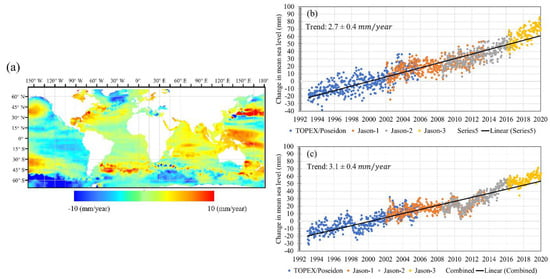
SL is an important oceanographic variable that should be measured precisely for long-term trend assessments and climate studies [44][205]. SL has a pivotal role in studies related to OSC, mesoscale eddies, and marine gravity fields [45][46][47][206,207,208]. In recent decades, anthropogenic activities and global warming have mainly resulted in SL change. For instance, the Intergovernmental Panel for Climate Change (IPCC) reported a Global Mean SL (GMSL) rise of 3.6 mm/yr between 2006 and 2015 [48][49][209,210]. However, the relative rate of SL change is not globally identical because it depends on different spatial and temporal parameters (see Figure 37).Figure 37. (a) Global SL change between 1993 and 2022. Regional mean SL changes and trends of (b) the Atlantic Ocean and (c) the Pacific Ocean calculated from a combination of TOPEX/Poseidon, Jason-1, Jason-2, and Jason-3 satellite altimetry datasets. Satellite altimetry data were downloaded from [50][211].
Table 4.
Different RS systems for SL Mapping along with their advantages and disadvantages.
| RS System (Passive/Active) | RS System (Type) | Advantage | Disadvantage |
|---|---|---|---|
| Passive | GNSS-R | Provides frequent all-weather data for regional to global studies | Requires data collected over a long period to enhance the accuracy of the SL estimation |
| Active | Altimeter | All-weather data acquisition with global coverage | Relatively coarse spatial resolution and low temporal resolution |
| Gravimeter | All-weather data acquisition, global coverage, and unique ocean mass measurements | Very coarse spatial resolution and unsuitable for regional studies |
3.5. Ocean Tide (OT)
. Ocean Tide (OT)
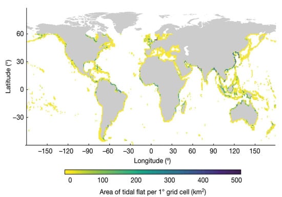
OT refers to the regular rise and fall of the ocean water caused by the gravitational pull of the moon and sun in relationship with the geometric location of the Earth’s surface [73][255]. The cyclical effects of the Earth’s and the moon’s rotations are, respectively, the primary factors of the periodic rhythm and height of OT [74][256], and 24 h and 50 min is the tidal period [74][256]. When the water wave slowly rises to its crest (highest level), covering much of the shore, high tide occurs. Once the water wave falls to its trough (the lowest part of the wave), it is known as low tide [73][74][255,256]. Thus, the tidal range is the vertical difference between the high and low OT [74][256]. Ebb tide is called the flow of water from high tide to low tide [73][255]. During the moon’s revolution around the Earth, the direction of its gravitational attraction is aligned with that of the Sun. High spring OTs are created when the moon, Earth, and sun are in alignment. This alignment occurs every 14–15 days during full and new moons [74][256]. On the other hand, during the first and last quarters of the moon, neap OTs happen when the moon appears half-full [73][74][255,256]. Intertidal zones are the lands in the tidal range categorized in the splash, high-tide, mid-tide, and low-tide zones [75][76][257,258]. While traditionally, in situ measurements and numerical models have been used for OT studies, RS has been proposed to fill OT measurement gaps over the past four decades. RS technology has expanded theour understanding of global OT [77][78][79][259,260,261] and facilitated continuous OT monitoring and predictions over wide-spread scales. RS systems can be used to study several aspects of OT, including tidal flats, tidal channels, tidal currents, Ocean Tidal Load (OTL), and tidal wetlands. In the following, a brief description of each type of OT is provided. The area inundated between low- and high-tide waterlines is defined as tidal flats and is a mixture of seawater and freshwater environments [80][262]. Tidal flats provide essential services, such as coastal storm protection, food production, and shoreline stabilization [80][262]. A recent study has discovered that tidal flats occupy approximately 130,000 km2 of the planet (Figure 48) [81][263]. Murray et al. [81][263] also reported that about 70% of the global tidal flats occurred in three continents, namely, Asia (44% of total), North America (15.5% of total), and South America (11% of total), 49.2% of which were concentrated in eight countries, namely, Indonesia, China, Australia, the United States, Canada, India, Brazil, and Myanmar. Monitoring tidal flats using field observations is limited to estimating the ebb/flood characteristics, adequate surveys for large tidal flats, and the field access. However, RS in combination with in situ measurements facilitates monitoring tidal flats in a more cost- and time-efficient approach. In fact, RS data with a high temporal resolution are necessary for tidal flats studies because there are coastal areas that fall dry during each tidal cycle [82][264], and tidal flats are only exposed fully for a short period at low tides.Figure 48.
Global distribution of tidal flats during 2014–2016. The figure is directly adopted from Reference [9].
Table 5.
Different RS systems for OT studies along with their advantages and disadvantages.
| RS System (Passive/Active) | RS System (Type) | Advantage | Disadvantage |
|---|---|---|---|
| Passive | Optical | Availability of open-access data, useful for all tidal applications, a wide range of spectral and spatial resolutions | Time and weather dependency, low accuracy in estimating water height changes |
| GNSS-R | NRT data, continuous data, independent from weather, cost-efficient | Sensitive to sea surface reflections, dependency on complementary data, applicable only to tidal channels and OTL | |
| Active | SAR | Accurate estimation of ocean surface topographic changes, independent from weather conditions and time, useful for all tidal applications | Complex processing steps |
| Altimeter | Multilook processing, accurate topographic measurements | Only global surface geostrophic, low track density, limited applications, applicable only to tidal channels and tidal flats | |
| LiDAR | Relatively higher spatial resolution, accurate estimation of ocean surface topographic changes | Comparatively costly, useful for the data acquisition at optimal tidal and weather conditions, insufficient coverage, applicable only to tidal channels, tidal flats, and tidal wetlands |
3.6. Ship Detection (SD)
. Ship Detection (SD)
SD has a wide variety of environmental, civil, and military applications. For example, the benefits of automatic locating and tracking ships for the civil sector are maritime management, vessel traffic services, safety and rescue, fishery management, and illegal fishery surveillance. Moreover, the main applications in the military sector include naval warfare, battlefield environment assessment, and pirate activity surveillance [93][94][95][313,314,315]. RS has a leading role in SD and monitoring because of its several advantages, such as the availability of open-access multitemporal datasets and large area coverage.Although various RS datasets have been used for SD (e.g., hyperspectral [96], TIR [97], and UAV [98] imagery), optical, SAR, and HF radar are the most common RS systems for SD [93].
Although various RS datasets have been used for SD (e.g., hyperspectral [316], TIR [317], and UAV [318] imagery), optical, SAR, and HF radar are the most common RS systems for SD [313]. Table 6
summarizes the main advantages and disadvantages of each of these systems for SD.
Table 6. Different RS systems for SD along with their advantages and disadvantages.
| RS System (Passive/Active) | RS System (Type) | Advantage | Disadvantage |
|---|---|---|---|
| Passive | Optical | Relatively high resolution | Functional only during the daytime, affected by clouds and weather condition |
| Active | SAR | Operational in all weather conditions and all times | Speckle noise, difficult interpretation |
| HF Radar | Operational in all weather conditions and all times | Lack of data availability due to the limited number of radars |
Figure 59.
A general ship detection method using spaceborne RS data.