1. Introduction

Time series data are a very common form of data, containing information about the (changing) state of any variable. Some common examples include stock market prices and temperature values across some period of time. Time series modeling tasks include classification, regression, and forecasting. There are unique challenges that come with modeling time series, given that measurements obtained in real-life settings are subject to random noise, and that any measurement at a particular point in time could be related to or influenced by measurements at other points in time [1]. Given this nature of time series data, it is impractical to simply utilize established machine learning algorithms such as logistic regression, support vector machine, or random forest on the raw time series datasets because these data violate the basic assumptions of those models. In recent years, two vastly different camps of time series classification techniques have emerged: deep-learning-based models vs non-deep-learning-based models. While deep learning models are extremely powerful and show great promise in classification performance and generalizability, they also present challenges in the areas of hyperparameter tuning, training, and model complexity decisions. 

2. Time Series Classification Techniques Used in Biomedical Applications

2.1. Preprocessing Methods

2.2. Feature Engineering Methods

Feature engineering is the most commonly used method of time series classification. The feature engineering pipeline usually consists of the following steps:

• Preprocessing: this step takes raw data as the input and performs some manipulation of the data to return cleaner signals. Common steps include artifact removal, filtering, and segmentation.
• Signal transformation: this step can be used in preprocessing and also as a precursor to feature extraction. Some manipulation is performed on the signal to represent it in a different space. Common choices are Fourier Transform and wavelet transforms.
• Feature extraction: in this step, features are extracted from the time series data as a new representation of the original time series.
• Feature selection: this step selects the features that are the most descriptive, or have the most explanation power. Feature selection is also frequently performed in conjunction with model building.
• Model selection: the best model is found through hyperparameter tuning and/or comparisons between different types of algorithms.
• Model validation: performance metrics are calculated for all of the final models. This is frequently done in conjunction with model selection and often using some form of cross-validation.

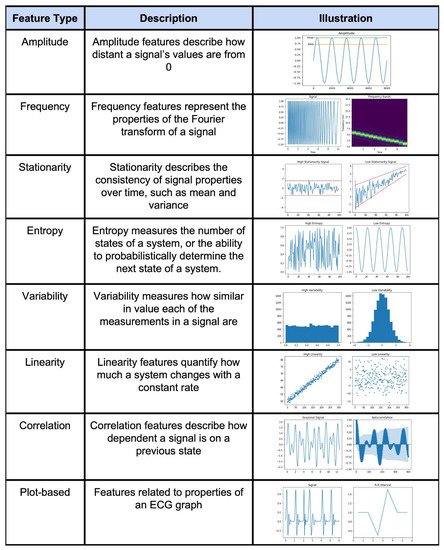
An example feature engineering technique for a time series is shown in Figure 14.  

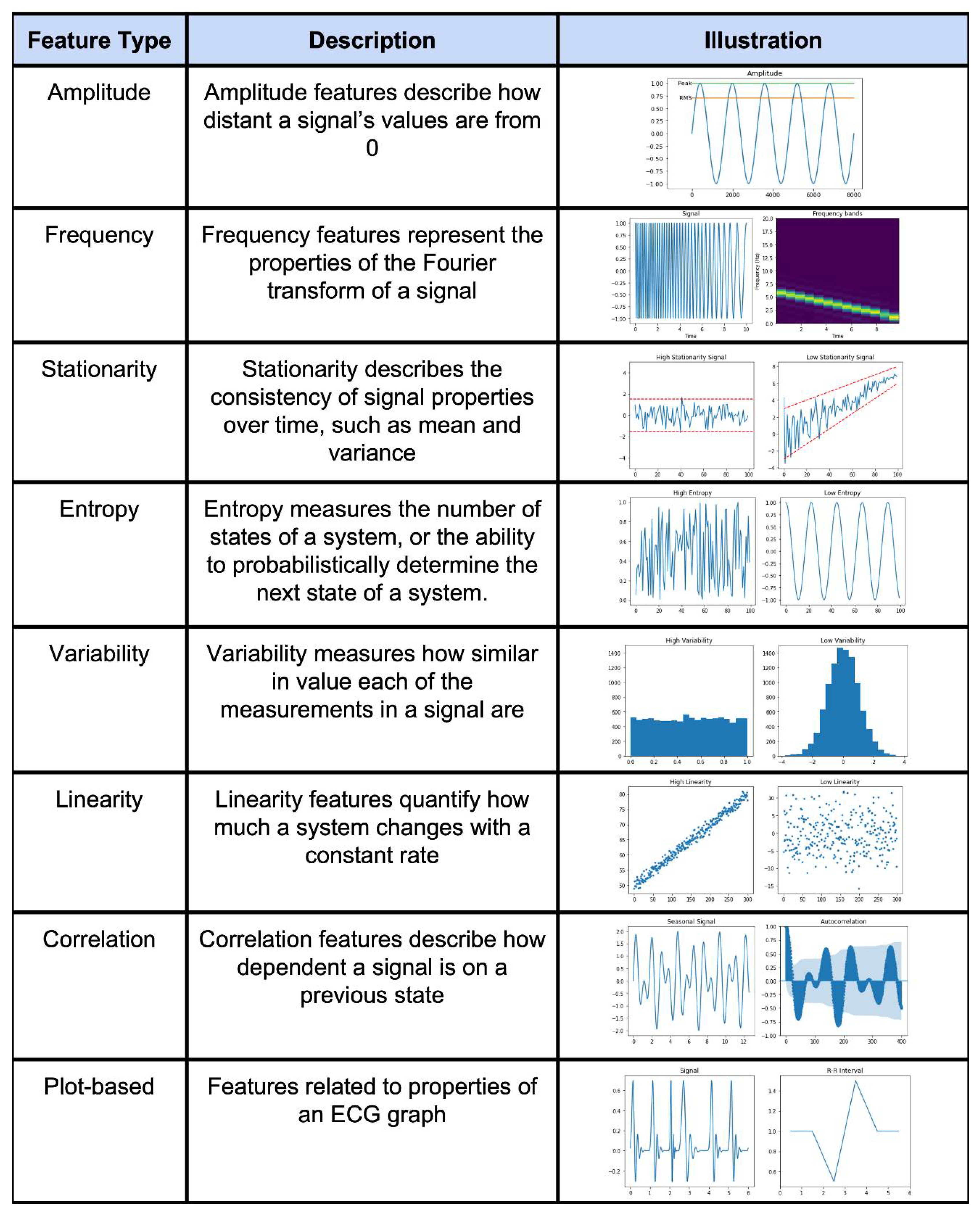
Figure 14. Illustration of different types of feature engineering techniques ^[9].

2.3. Other Methods

Ensemble Methods: Ensemble-based methods are characterized by the connection of multiple algorithmic models that join forces to make the final prediction. These methods may or may not need an additional feature engineering step. Some algorithms that do not necessitate feature engineering in this category are Hierarchical Vote Collective of Transformation-based Ensembles and Bag of Symbolic Fourier Approximation Symbols ensemble algorithms (BOSS) ^[10].

State-space Models: State-space models are characterized by the construction of a state and transition model where the transitions are modeled by probabilities. Often, state-space models are most intuitively used for sequence-to-sequence or point-wise classification. For example, She et al. ^[11] introduced an adaptive transfer learning algorithm to classify and segment events from non-stationary, multi-channel temporal data recorded by an Empatica E4 wristband, including 3-axis accelerometry (ACC), blood volume pulse (BVP), skin temperature (TEMP), and electrodermal activity (EDA). Using a multivariate Hidden Markov Model (HMM) and Fisher’s Linear Discriminant Analysis (FLDA), the algorithm adaptively adjusts to shifts in the distribution over time, thereby achieving an accuracy of 0.9981 and F1-score of 0.9987. 

Illustration of different types of feature engineering techniques [30].

2.3. Other Methods

Ensemble Methods: Ensemble-based methods are characterized by the connection of multiple algorithmic models that join forces to make the final prediction. These methods may or may not need an additional feature engineering step. Some algorithms that do not necessitate feature engineering in this category are Hierarchical Vote Collective of Transformation-based Ensembles and Bag of Symbolic Fourier Approximation Symbols ensemble algorithms (BOSS) [13].

State-space Models: State-space models are characterized by the construction of a state and transition model where the transitions are modeled by probabilities. Often, state-space models are most intuitively used for sequence-to-sequence or point-wise classification. For example, She et al. [33] introduced an adaptive transfer learning algorithm to classify and segment events from non-stationary, multi-channel temporal data recorded by an Empatica E4 wristband, including 3-axis accelerometry (ACC), heart rate (HR), skin temperature (TEMP), and electrodermal activity (EDA). Using a multivariate Hidden Markov Model (HMM) and Fisher’s Linear Discriminant Analysis (FLDA), the algorithm adaptively adjusts to shifts in the distribution over time, thereby achieving an accuracy of 0.9981 and F1-score of 0.9987. 

Shape/Pattern-based: These models are characterized by mining or comparing shapes or patterns in a time or sequence vector. For example, Zhou et al. [35] published an algorithm that can take into consideration the interaction among signals collected at spatiotemporally distinct points, where fuzzy temporal patterns are used to characterize and differentiate between different classes of multichannel EEG data. This algorithm achieved an accuracy of 0.9318 and an F1-score of 0.931, thereby classifying positive vs negative emotion states. Distance-based: These models calculate the distance (or differences) of time series data vectors. For example, Forestier et al. [36] propose an efficient algorithm to find the optimal partial alignment (optimal subsequence matching) and a prediction system for multivariate signals using maximum a posteriori probability estimation and filtering. This scoring function is based on dynamic time warping. They were able to achieve an accuracy of 0.95, an F1-score of 0.926, and a sensitivity of 0.896.

Shape/Pattern-based: These models are characterized by mining or comparing shapes or patterns in a time or sequence vector. For example, Zhou et al. ^[12] published an algorithm that can take into consideration the interaction among signals collected at spatiotemporally distinct points, where fuzzy temporal patterns are used to characterize and differentiate between different classes of multichannel EEG data. This algorithm achieved an accuracy of 0.9318 and an F1-score of 0.931, thereby classifying positive vs negative emotion states.

Other: There are other methodologies that are difficult to characterize. One common method is performed by using statistical modeling of some sort. For example, İşcan et al. [37] published a high performance method to classify and discriminate various ECG patterns (to identify and classify QRS complexes). The model is called LLGMN, which is composed of a Log-Linear Model and a Gaussian Mixture Model (GMM), and gives a posterior probability for the training data. This model was able to achieve the highest accuracy, which was 0.9924.

Distance-based: These models calculate the distance (or differences) of time series data vectors. For example, Forestier et al. ^[13] propose an efficient algorithm to find the optimal partial alignment (optimal subsequence matching) and a prediction system for multivariate signals using maximum a posteriori probability estimation and filtering. This scoring function is based on dynamic time warping. They were able to achieve an accuracy of 0.95, an F1-score of 0.926, and a sensitivity of 0.896.

Another common method is designing a composite metric or index based on domain knowledge or data-driven metrics. For example, Zhou et al. [38] proposed a new algorithm to detect gait events on three walking terrains in real-time based on an analysis of acceleration jerk signals with a time–frequency method to obtain gait parameters, as well as detecting the peaks of jerk signals using peak heuristics. The performance of the newly proposed algorithm was evaluated in eight healthy subjects walking on level ground, upstairs, and downstairs. The mean F1-score was above 0.98 for HS (heel-strike) event detection and 0.95 for TO (toe-off) event detection on the three terrains.

Other: There are other methodologies that are difficult to characterize. One common method is performed by using statistical modeling of some sort. For example, İşcan et al. ^[14] published a high performance method to classify and discriminate various ECG patterns (to identify and classify QRS complexes). The model is called LLGMN, which is composed of a Log-Linear Model and a Gaussian Mixture Model (GMM), and gives a posterior probability for the training data. This model was able to achieve the highest accuracy, which was 0.9924.

2.4. Interpretation Methods

Another common method is designing a composite metric or index based on domain knowledge or data-driven metrics. For example, Zhou et al. ^[15] proposed a new algorithm to detect gait events on three walking terrains in real-time based on an analysis of acceleration jerk signals with a time–frequency method to obtain gait parameters, as well as detecting the peaks of jerk signals using peak heuristics. The performance of the newly proposed algorithm was evaluated in eight healthy subjects walking on level ground, upstairs, and downstairs. The mean F1-score was above 0.98 for HS (heel-strike) event detection and 0.95 for TO (toe-off) event detection on the three terrains.

2.4. Interpretation Methods

Model interpretability is a significant aspect of model building. In time series classification for biomedical applications, the interpretation of models that have been built and validated could highlight potential insights into the biomedical phenomenon of interest. Some models have a built-in methodology of interpretation, such as statistical modeling (Hidden Markov Models, Bayesian Models, or ARIMA models) and indices that are informed based on domain knowledge. For many more models with great performance, however, interpretability is a challenge.

2.5. Best Performing Algorithms

Overall, the statistical modeling classifiers and feature engineering methods performed the best and most consistently for all input signal types. Wavelet transformation iwas consistently and widely used and achieving great performances as a used as a preprocessing method, feature extraction method, or as an integral part of index development, and furthermore, that it achieved great results.

3. Conclusions

In conclusion, non-deep learning time series classification techniques can achieve competitive performances, while also allowing for great interpretability. However, this field still lacks standardization for model testing, validation procedures, and reporting metrics, which should be addressed to allow for better reproducibility and understanding of the  presented algorithms.