Your browser does not fully support modern features. Please upgrade for a smoother experience.
Please note this is a comparison between Version 1 by Antimo Cagnotta and Version 3 by Catherine Yang.
Jet Flavour Tagging briefly describes the main algorithms used to reconstruct heavy-flavour jets. Jet Substructure and Deep Tagging focuses on the identification of heavy-particle decay in boosted jets. These so-called tagger algorithms have a relevant role in physics studies since they allow researchers to successfully reconstruct and identify the particles that caused the jet and, in some cases, allow analyses that would otherwise be unfeasible.
- machine learning
- jet tagging
- particle physics
1. The CSVv2 Tagger
Heavy-flavour jet tagging is linked to the properties of the heavy-hadrons in the jets. The CSVv2 algorithm is based on the CSV algorithm; however, displaced track information is combined with the relative secondary vertex as input for multivariate analysis. A feed-forward multilayer perceptron with one hidden layer is trained to tag the b-jet. The jet’s PpT and η distributions are reweighted in order to have the same spectrum for all the jet flavours in the training, thereby avoiding discrimination based on the spectrum of these variables, which would introduce a dependence on the sample used. Three different jet categories are defined based on the number and type of secondary vertices reconstructed: RecoVertex, PseudoVertex, and NoVertex. The values of the discriminator of the three categories are combined with a likelihood ratio that takes into consideration the fraction of jet flavour derived in a sample composed of top quark–antiquark (tt¯) events. Moreover, two different trainings are performed with c-jets and light-jets as the background. The final value of the discriminator is the weighted average of the two training outputs, with a relative weight of 1:3 for c-jet to light-jet trainings. The CSVv2 algorithm by default uses vertices reconstructed with the IVF algorithm, but it has also been studied with AVR reconstruction, and this is referred to as CVSv2 (AVR). Figure 12 shows the output of the two versions of the CSVv2 algorithm.
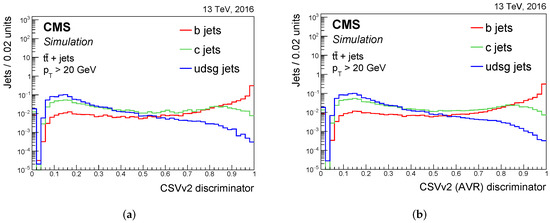
Figure 12. Distribution of the CSVv2 discriminant for jets of different flavour in tt¯ events: the output for the version with (a) IVF reconstruction and with (b) AVR reconstruction. The distributions are normalised to unit area. Jets without a selected track and secondary vertex are assigned a negative discriminator value. The first bin includes the underflow entries [1][18].
2. The DeepCSV Tagger
The DeepCSV algorithm was developed with a Deep Neural Network (DNN) with more hidden layers and more nodes per layer in order to improve the CSVv2 b-tagger. The input is the combination of the IVF secondary vertices and up to the first six track variables, taking into consideration all the jet-flavour and vertex categories. Variable preprocessing is used to speed up training and centres the distributions around zero with a root mean square equal to one. The jet pT range used in training goes from 20 GeV up to 1 TeV and remains within the tracker acceptance by also using the preprocessed jet pT and η as input.
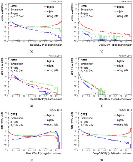
The neural network, developed with KERAS [2][20], uses four fully connected hidden layers, and each layer has 100 nodes. The activation function of each node is a rectified linear unit that defines the output of the node, with the exception of the last layer, for which the output is a normalised exponential function interpreted as the probability of flavour f of the jet (P(f)). Five jet categories corresponding to the nodes in the output layer are defined: one for b hadron jets, at least two for b hadrons, one for c hadron and no b hadron, at least two for c hadron and no b hadron, and other jets. Figure 23 shows the DeepCSV probability P(f) distributions.
The DeepCSV tagger is used also for c tagging, which combines the probabilities corresponding to the five categories. In particular, the DeepCSVCvsB discriminant is used to discriminate c jets from b jets and is defined as:
and the denominator is the probability of identifying a c jet or a light jet.
$DeepCSVCvsB = \frac{P(c)+P(\ccbar)}{1-P(udsg)}, $
where 1−P(usdg) is the probability of identifying an a, b, or c jet. In the same way, DeepCSVCvsL is defined to discriminate c jets from light jets:
DeepCSVCvsL=P(c)+P(
c\bar{c}
)1−(P(b)+P(bb¯)),
3. The DeepJet Tagger
Recently, a new network architecture was developed: the DeepJet tagger [3][21]. Different from CSVv2 and DeepCSV taggers, this architecture examines all jet constituents simultaneously. The DeepJet algorithm uses a large number of input variables that can be categorised into four groups: global variables (jet kinematics, the number of tracks in the jet, etc.), charged and neutral PF candidates, and variables of the SVs related to the jet. For the same reasons seen in Section 2.1, the jets pT and η are reweighted during data preprocessing to avoid discrimination closely related to the kinematic domain used during training.
The basic idea in the DeepJet architecture is to use low-level information from all subjet features. In order to process an input variable space of such dimensions, the architecture needs an appropriate training procedure. Four separate branches are used in the first step: all four of the groups listed above except the global variables are filtered through a 1×1 convolutional layer. Each of the three outputs is then processed into a recurrent layer of the Long Short-Term Memory (LSTM) type [4][22]. The three LSTM outputs are collected with the global variables and then input in a fully connected layers. In order to discriminate between b-tagging, c-tagging, and quark/gluon tagging, the six output nodes of the previous layers are integrated into a multi-classifier.
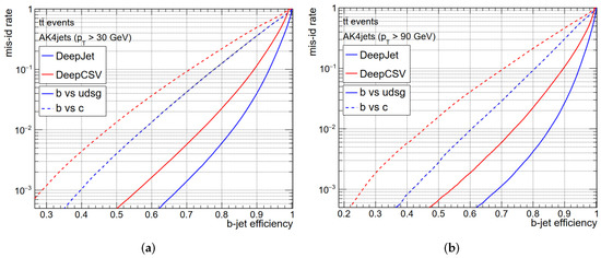
Training is performed using the Adam optimiser with a learning rate of 3×10⁻⁴ for 65 epochs and categorical cross entropy loss. The learning rate is halved if the validation sample loss stagnates for more than 10 epochs. In Figure 34, the Receiver–Operative Characteristic (ROC) curves for two different pT ranges for the same dataset are reported and compared to the performance of the DeepCSV tagger. Such curves display the background misidentification efficiency versus the signal efficiency measured from Monte Carlo simulation.