Your browser does not fully support modern features. Please upgrade for a smoother experience.
Please note this is a comparison between Version 1 by Basit Qureshi and Version 3 by Catherine Yang.
In IoT sensor networks, wireless communication protocols are popularly used for the information exchange process. These communication protocols work as unlicensed frequency bands that ease the flexibility and scalability of sensor deployments. However, the utilization of communication protocols for wireless sensor network (WSN) under unlicensed frequency bands causes uncontrollable interference. The interference signals may lead to improper data transmission and sensor data with noise, missing values, outliers and redundancy.
- Internet of Things
- data processing
- data analysis
- data fusion
1. Denoising
The voluminous sensor data generated in the IoT network needs data analysis, mostly with real-time decision-making. The characteristics of sensor data are complex, involving high velocities, huge volumes, and dynamic values and types. Further, the sensor data pollute while perpetuating numerous obstacles until producing the required data analysis and real-time decision-making.
Noise is an uncorrelated signal component that enacts unwanted change and modification on the original vectors of the signal. The noise feature leads to the unnecessary processing and utilization of resources for handling the unusable data. The wavelet transform methods are capable of representing the signal and addressing the problem of signal estimation effectively. Significantly, the wavelet transformation preserves the original signal coefficients by removing the noise within the signal. This is achieved by thresholding the coefficient of noise signals, hence the perfect thresholding scheme is essential. The wavelet transformation is a prevalent method to analyze and synthesize continuous-time signal energy.
Let e(t), t ∊ R represent the signal energy, while it must satisfy the constraint defined as
where the signal energy e(t) that satisfies the constraint in Equation (1) belongs to the squared search space L2(R). The wavelet transformation is also used to analyze the discrete-time signal energy and eliminate the noise with energy signals. The wavelet transformation method allows us to investigate the signal characteristic by zooming at different time scales. The experimental results exhibited significant improvements in denoising the sensor signals.
There are two types of wavelet transforms, namely Continuous Wavelet Transform (CWT), which targets signal analysis on a time-frequency level, and Discrete Wavelet Transform (DWT) that targets signal analysis a time level.
Continuous Wavelet Transform (CWT): In CWT, the signal energy e(t) is represented using a set of wavelet functions C={Wψ(α,β)},α∈R+;β∈R, where α represents the dilation scaling factor, and β represents the shifting time localization factor, while ψ represents the wavelet function. The wavelet coefficient on the time-frequency plane is given by Equation (2).
where ψ0 represents the shifted and dilated form of the original wavelet ψ0(t). The CWT is a function controlled by two parameters. The CWT targets to find the coefficients of the original signal e(t) based on the shifting factor (β) and the dilation factor (α).
Discrete Wavelet Transformation (DWT): The DWT for continuous-time signals refers to transforming signals performed upon a discrete-time signal. The coefficients obtained from this transformation are defined in subset D=Wψ(2α,2αβ),α∈Z, β∈Z. For a given continuous-time signal e(λ), the coefficients of DWT are obtained using the integration of the subset D, as defined in Equation (3).
where α indicates the scale factor and β indicates the localization factor. It is to be noted that this involves continuous-time signal e(λ), and not the discrete signal.
The authors in [1][24] discuss that in some instances the signals received from the IoT sensor devices have a reasonable ratio value of Signal to Noise (SNR), but are unable to achieve the required Bit Error Rate (BER). To overcome such problems, the best solution is to eliminate the inferior wavelet coefficients. This elimination improves the SNR, based on a specific threshold limit. This is possible as the smaller coefficients tend towards more noise data than the desired signal data. Further, it is to be noted that the energy signals are concentrated on a particular part of the signal spectrum. As such, if that specific part of the signal spectrum has been transformed using wavelet coefficients, it improves the SNR value. Further, if the signal function has large regions of irregular noise and small smooth signal regions, then the wavelet coefficients play a vital role in improving the signal energy. Thus, if any signal function is polluted by larger noise, the wavelet coefficients are affected in the more significant part of the wavelet coefficients. The original signal will be contained within the small parts of wavelet coefficients. Thus, maintaining the right threshold limit would eliminate the majority of noise signals and retain the original signal coefficients. In this paper, the authors elaborate on the streaming of sensor data and raw sensor signals to recognize the characteristics and various issues related to noise associated with the sensor signals.
2. Missing Data Imputation
Imputation is an essential pre-processing task in data analysis for dealing with incomplete data. Various fields and industries like smart cities, healthcare, GPS, smart transportations, etc., use the Internet of Things as a key technology that generates lots of data [2][25]. The learning algorithms which analyze the IoT data generally assume that the data are complete. While missing data are common in IoT, the data analytics performed on missing or incomplete IoT data may produce inaccurate or unreliable results. Therefore, an estimate of the missing value is necessary for IoT. Three main tasks must be performed to solve this problem. The first step is finding the reason for missing data. Poor network connectivity, faulty sensor systems, environmental factors and synchronization issues are the various reasons for the incomplete results. The missing data are divided into three types: missing completely at random (MCAR), missing at random (MAR), and not missing at random (NMAR). The further step involves studying the pattern of missing data. The two approaches are monotonous missing patterns (MMP) and random missing patterns (AMP). Finally, they form a missing value imputation model for IoT to use the model to approximate the value for the missing data. Within the literature, some missing value imputation algorithms include single imputation algorithms, multivariate imputation algorithms, etc. The traditional imputation algorithm is not suitable for IoT data. There are some algorithms which are mainly used for missing data imputation, and these are given in the next section.
Gaussian Mixture model: The Gaussian Mixture Model (GMM) is a clustering algorithm [3][26]. It is a probabilistic model that uses a soft clustering approach for distributing the data points to different clusters.
A Gaussian Mixture is defined as follows: G = {GD1, GD2, …, GDk}, where k denotes the number of clusters. Each GDi is a Gaussian distribution function that comprises a mean μ, which represents its center, a covariance Σ, and a probability π, which denotes how big or small the Gaussian function will be. Assuming a data set D is generated using GMM with k components, the function fk (GDi) represents the probability density function of the kth component. The probability of GDi, P(GDi) generated by GMM, is as given in Equation (4) below.
To handle the missing data imputation of the IoT sensor data using the GMM model involves five steps, namely instance creation, clustering, classification, distance measuring and data filling. First, the instances in the data set D are divided into two separate data sets, as D1 and D2. D1 contains all the instances without missing values, whereas D2 contains all instances in the data set which has the missing values. Secondly, the GMM model based on the EM algorithm is used to cluster the complete data set D1. The cluster center for each cluster is determined. After that, the cluster for each instance in D1 is computed. Third, the incomplete data set D2 is taken as a testing set. Each instance in D2 is classified according to the clustering result. For instance, αi ∈D2, αi belongs to a cluster if it is closer to the cluster center of that cluster by Euclidean distance. In the fourth step, for each instance αi in D2, one must determine one or more complete instances that are closest to αi in the same cluster, using Euclidean distance as the distance measure. Finally, one must fill in the missing value of the instance αi by finding the mean value of the closest instance in the cluster.
Spatial and temporal correlation [4][27]: Sensor nodes periodically detect data. Since the sensor data are time-sensitive, different results would be obtained using other sensor data for analysis. The relationship between the sensor nodes in different periods is not the same, so it is necessary to select the correct data to analyze. According to authors, the appropriate sampling of data is required for accurate data analysis. The authors propose the Temporal and Spatial Correlation Algorithm (TSCA) to estimate the missing data. Firstly, it saves all the sensed data simultaneously as a time series and selects the most important series as the analysis sample, which significantly improves the algorithm’s efficiency and accuracy. Secondly, it estimates missing temporal and spatial dimensional values. These two measurements are assigned different weights. Third, there are two strategies for dealing with severe data loss, which boosts the algorithm’s applicability. The basic workflow of the TSCA model is illustrated in Figure 12.
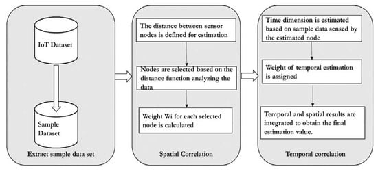
Figure 12. The workflow of the Temporal and Spatial Correlation Algorithm.
The model as illustrated in Figure 12 assumes all the sensors are in the same communication range. The experiment was conducted on the air quality data set. As a first step, the target data set is extracted from the original data set. A missing data threshold is set, which differs from case to case. In the next step, compute the percentage of missing values. If it exceeds the threshold, then the imputation is ignored; otherwise, the spatial–temporal imputation is carried out. In the next step, the n proximity sensors are computed using the Haversine distance formula. The correlation between the n proximity sensors and the sensor with a missing value is calculated using the Pearson correlation co-efficient. Finally, the complete target data set is constructed and evaluated for accuracy.
The authors in [5][28] suggested a novel method of nearest neighbor imputation to impute missing values based on the spatial and temporal correlations between sensor nodes. The data structure kd-tree was deployed to boost search time. Based on the percentage of missing values, weighted variances and weighted Euclidean distances were used to create the kd-tree. Figure 23 illustrates the workflow of the spatial–temporal model. The algorithm defined in the proposed model follows the steps, as firstly, it sets the missing value threshold as T. The percentage P of the missing values in the chosen data set is then calculated. If P is within the threshold, then it finds the n proximate sensors through spatial correlation. The correlation between the sensors with the missing values and the n proximity sensors is computed using the Pearson correlation coefficient. The missing sensor data are then imputed by the readings of the proximity sensors corresponding to the time. The output data set is completed. The result is then compared with multiple imputation outcomes. Again, the accuracy is evaluated using Root Mean Square Error (RMSE).
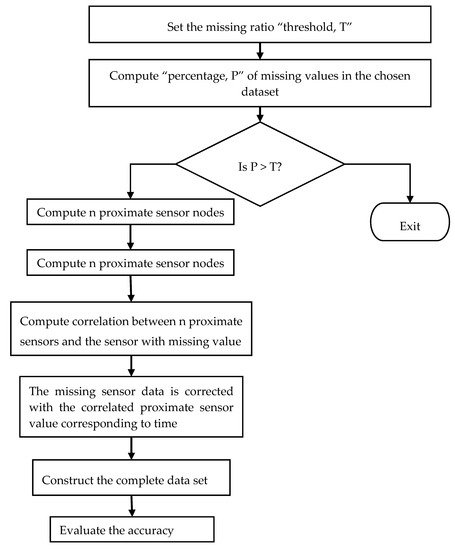
Figure 23. The workflow of the spatial–temporal model.
Incremental Space-Time Model (ISTM): The incremental model discussed in [6][29] is the model that updates the parameters of the existing model depending on the previous incoming data, rather than constructing a new model from scratch. The model uses incremental multiple linear regression to process the data. When the data arrive, this model is updated after reading the intermediary data matrix rather than accessing all the historical data. If any missing data are found, then the model provides an estimated value based on the nearest sensors’ historical data and observations. The working of the ISTM model has three phases, which are initialization, estimation and updating. In the initialization phase, the model is initialized with historical data. For each sensor p, the historic data and the recording reference are represented as a data matrix. It also computes two intermediary matrices using these data matrices. Next, in the estimation phase, if the sensor’s data contain one missing value, then the model generates an estimated value in real-time. It does this by referring to some data in the database. The estimated value will be then saved in the database. Finally, if the data arriving from the sensor do contain any missing value in the updating phase, then the model updates the new data. It then stores this in a reference database.
Probabilistic Matrix Factorization: There are two major advantages of using probabilistic matrix factorization (PMF) [7][30] for handling missing IoT sensor data. First is the dimensionality reduction, which is the underlying property of matrix factorization. The second is that the original matrix can be replicated using the factored matrices product. This method is used to recover the values missing in the original matrix. PMF is performed on the preliminarily assigned sensors. The neighboring sensors’ data are examined for similarity, and are grouped into a different class of clusters using the K-means algorithm.
The K-means clustering algorithm groups the sensors into separate classes according to their measuring similarity. Analyzing the patterns of neighboring sensors helps to recover missing sensor data. Then, a probabilistic matrix factorization algorithm (PMF) is implemented in each cluster. PMF standardizes the data and restricts the probabilistic distribution of random features. The workflow of the algorithm is illustrated in Figure 34.
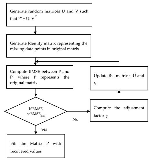
Figure 34. The workflow of the PMF model.
In the algorithm, PMF is used to factorize a single matrix into the product of two matrices. The dimensionality can be reduced by factorization. The ability to obtain the original matrix from the product of two factored matrices can be used to recover the missing values in the original matrix. The original matrix is represented as P NxM. Now generate two random matrices, U and V, such that P’ = U. V T, where U and V are of dimension NxK and KxM, respectively. K is an integer which represents the number of latent feature column-vectors in U and V. The missing data points in the original matrix are represented as an identity matrix, I having the same dimension as the original matrix P. The values in the Iij matrix are defined using the following rule, as depicted in Equation (5).
Next, compute the root mean square error (RMSE) between the P and P’, which is given in Equation (6) below.
The result obtained using Equation (1) is compared with RMSEmax, which is the maximum acceptable error. The algorithm will terminate if RMSE is ≤ RMSEmax. Otherwise, the values of U and V are updated using the Equations (7) and (8).
where γ denotes the adjustment factor that decides how much the U and V values need to be adjusted. Steps four to six are repeated until the RMSE is less than or equal to RMSEmax. A large value of γ may result in low precision, while a value that is too small may result in too many iterations.
The authors in [8][31] addressed the issue of missing value in IoT sensors. In IoT sensor networks, single-mode failures cause data loss due to the malfunction of several sensors in a network. The authors proposed a multiple segmented imputation approach, in which the data gap was identified and segmented into pieces, and then imputed and reconstructed iteratively with relevant data. The experimental results exhibited significant improvements over the conventional technique of root mean square.
3. Data Outlier Detection
In the IoT sensor network, the sensor nodes are widely distributed and heterogeneous. It is to be noted that, in a real physical environment, such a setup leads to enormous failure and risks associated with sensor nodes due to several external factors. This causes the original data generated from the IoT sensor network to become prone to modifications and produce data outliers [9][32]. Therefore, it is essential to identify such data outliers before performing data analysis and decision-making. For this purpose, spatial correlation-based data outlier detection is performed and carried using three popular methods, namely majority voting, classifiers, and principal component analysis.
Voting Mechanism: In this method, a sensor node is identified as functioning abnormally by finding the differences in reading with neighboring sensor nodes. According to authors [10][33], the Poisson distribution is the usual data generation method in various IoT sensor network applications. In the IoT sensor network, the data sets generated consist of outliers for short-term, non-periodic, and insignificant changes in data trends. The simple and efficient statistical methods for outlier detection in the Poisson distribution of the IoT sensor network data set are standard deviation and boxplot. Similarly, in a distributed environment, the Euclidean distance is estimated between the data generated by the faulty sensor node and the data from its immediate neighbor nodes. If the estimated difference in the data exceeds a specific threshold limit, then the data generated by this node are identified as an outlier. Although this technique is simple and less complicated, it is excessively dependent on the neighboring sensor nodes. Furthermore, the accuracy in the case of the sparse network is low.
Classifiers: This method involves two steps, firstly training the IoT sensor data using a standard machine learning model. Secondly, the data are detected using the classifier algorithms as either normal or anomaly [11][34]. The commonly used classifier algorithms is the support vector machine (SVM). Half of the data search space is trained to be standard data. Later, the data are analyzed and classified through SVM for the detection within the trained data of standard data, or otherwise of abnormal data. However, the demerits of the classifier algorithm involve its high complexity in the computation aspect.
Principal Component Analysis (PCA): The objective of PCA is to identify the residual value by extracting the principal components of the given data set. The residual values estimated by the data are evaluated through detection mechanisms such as T2 score and squared prediction error (SPE) to identify the data outliers.
In [12][35], the authors addressed the outlier detection in the IoT sensor data using the Tucker machine and the Genetic Algorithm. Different sensor nodes are involved in the IoT sensor network, exhibiting spatial attributes and sensing data. Furthermore, the sensor data generated are dynamic for the time. Generally, the extensive sensor data contain anomalies due to the mode failure. The conventional means of detecting outliers involves vector-based algorithms. The demerits of vector-based algorithms disturb the original structural information of the sensor data, and exhibit the side effect of dimensionality. The authors proposed a tensor-based solution for the outlier detection using tucker factorization and genetic algorithms. The experimental results demonstrated improvements in the efficiency and accuracy of outlier detection without disturbing the intrinsic sensor data structure.
4. Data Aggregation
The data aggregation method is referred to as the method that collects and communicates information in a summary form. This can be used for statistical analysis. In IoT, heterogeneous data are collected from various nodes. Sending data separately from each node leads to high energy consumption, and needs a high bandwidth across the network, which reduces the lifetime of the network. Data aggregation techniques prevent these kinds of problems by summarizing data, which reduces the excessive transfer of data, increases the network’s lifetime, and reduces network traffic. Data aggregation in the Internet of Things (IoT) helps to decrease the number of transmissions between objects. This lengthens the lifetime of the network and decreases energy consumption [13][36]. It also reduces network traffic.
The data aggregation methods in IoT are classified into the following:
- (a)
-
Tree-based approach [14][15][16][17][18][19][20][37,38,39,40,41,42,43]—This approach deploys the nodes in the network in the form of a tree. Here, the hierarchical and intermediate nodes perform the aggregation. The aggregated data are then transferred to the root node. The tree-based approach is suitable for solving energy consumption and lifetime of network problems;
- (b)
-
Cluster-based approach [21][22][23][24][25][44,45,46,47,48]—The entire network is organized as clusters. Each cluster will contain several sensor nodes with one node as the cluster head, which performs the data aggregation. This method aims to carry out the effective implementation of energy aggregation in large networks. This helps to reduce the energy consumption of nodes with limited energy in huge networks. Therefore, it results in a reduced overhead bandwidth due to the transfer of a limited number of packets. In the case of static networks where the cluster structure does not shift for a long time, cluster-based techniques are successful
- (c)
The authors in [28][51] addressed the issue of data uncertainty in IoT sensor data. Mainly, the data aggregation focused on device to device communication. The proposed technique involves the reconstruction of subspace-based data sampling. Next, the low-rank approximation is performed to identify the dominant subspace. Further, the robust dominant subspace is utilized for reliable sensor data, in an entirely supervised manner. The proposed method exhibits improvements in terms of accuracy and efficiency as regards removing the uncertainties and data aggregation of sensor data from the experimentation results.