Your browser does not fully support modern features. Please upgrade for a smoother experience.
Please note this is a comparison between Version 1 by SangHyun Joo and Version 2 by Dean Liu.
eDenoizer effectively orchestrates both the denoizer and the model defended by the denoizer simultaneously. In addition, the priority of the CPU side can be projected onto the GPU which is completely priority-agnostic, so that the delay can be minimized when the denoizer and the defense target model are assigned a high priority.
- IoT edge device
- embedded GPU
- approximate computing
- tucker decomposition
1. Solution Overview
Figure 15 details the operational workflow of eDenoizer. A rough look at the proposed approach shows that it consists of the offline procedure and the run-time one. In offline, DUNET is approximated through Tucker decomposition. Next, after performing training through the post hoc fine-tuning step, the accuracy loss is minimized and DUNETD is obtained. In run-time mode, multiple deep learning models and DUNET are executed over a scheduling framework, which consists largely of a set of DNN model threads, a job queue, and a kernel launcher. DNN model threads are composed of deep learning models, each of which is implemented as a thread and is a target scheduled to the CPUs over the underlying OS (operating system). Each model thread can asynchronously request its own DNN operation to the job queue. The kernel launcher extracts the requested operation from the job queue through the worker threads that exist inside it and enqueues it to the EE queue of the GPU.
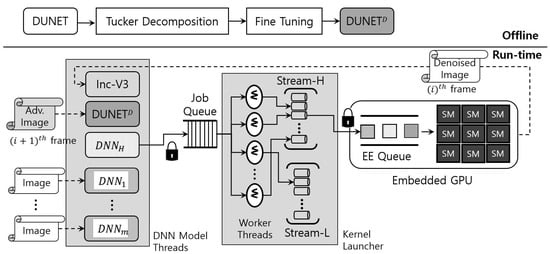
Figure 15.
Operational workflow of eDenoizer.
The computational output from the GPU is the result of the requested operation of a DNN model, including DUNET, which is mainly feature map data (mostly an intermediate result). This value is stored in the system memory, fed back to the set of DNN model threads, and then input to the corresponding model. At this time, if the result value is a denoize image, which is the final output of DUNET, it is not given as a DUNET input again, but as an input to the DNN model (e.g., Inception-V3 [1][20] in Figure 15) that performs target inference.
IAs mentioned earlier in Section 3, if DUNET does not finish its denoizing step for the (i)th image, the (i)th target inference step cannot occur. In addition, the (i+1)th DUNET processing step and the (i)th target inference step have no data dependency. Thus, as shown in Figure 15, both can be handled asynchronously and simultaneously in the scheduling framework. It is noteworthy that, and as described above, since the processing of DUNET was shortened with Tucker decomposition, the total target inference time is only bounded by the target inference time (i.e., (i+1)th DUNET step is hidden by (i)th target inference).
2. Scaling down the Computational Scale of DUNET
TAs detailed in Figure 4, the first hurdle reswearchers want to overcome is to maximize ΔAi. To do so, Reswearchers shrink the computational complexity of the original DUNET by applying an approximate computing method using Tucker decomposition, and Figure 36 describes the result of it. Since the four circles drawn with dashed lines in Figure 2 take over more than 40% out of the total amount of computations, those 3 × 3 convolutional layers need to be changed to have a structurally small computational quantity. Each of the four convolutional layers in Figure 2 is changed into two 1 × 1 convolutional layers and one smaller 3 × 3 convolutional layer, and the four black boxes with ‘TD’ in white letters in Figure 36 imply those Tucker-decomposed convolution kernel tensors.
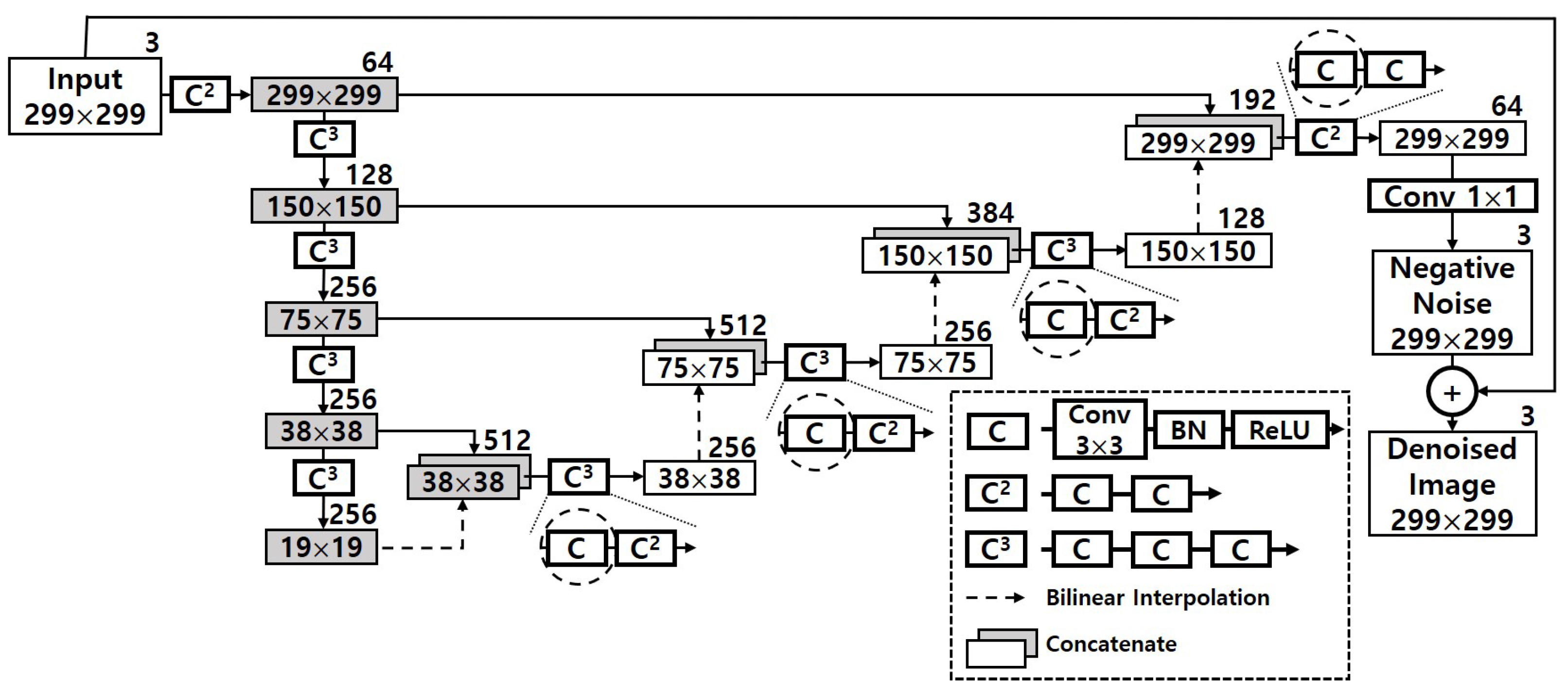
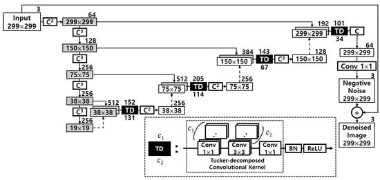
Figure 36. Approximate DUNET via Tucker decomposition.
To take advantage of dimension reduction, the two 1 × 1 convolutional layers (the two factor matrixes in Figure 3) are given to the both sides of the 3 × 3 convolutional layer (the core tensor), which is the same as the bottleneck building block in ResNet-152 [2][21]. The numbers above each black box represents the number of the output channel in each first 1 × 1 Tucker-decomposed convolution kernel tensor, and the numbers below represents the number of the output channel of the 3 × 3 core tensor which is immediately adjacent to the first 1 × 1 kernel tensor. The total computation volume is reduced by changing the number of large output channels pointed out in Figure 2 to c1 and c2.
For instance, the left first circle drawn with dashed line in Figure 2 has one 3 × 3 kernel tensor with 256 output channels. As shown in Figure 3, it is decomposed into three small convolution tensors, and the number of the output channel of each tensor is 152, 131, and 256, respectively. To explain this more clearly and quantitatively, researchers analyze the reduced computation amount, and that part is shown again in Figure 47. The computational cost of one convolutional layer is obtained by the formula shown in the figure. It can be seen that the convolutional layer, which originally had an arithmetic amount of kh×kw×ci×co×wo×ho = 3 × 3 × 512 × 256 × 38 × 38 = 1,703,411,712, is reduced to 1 × 1 × 512 × 152 × 38 × 38 + 3 × 3 × 152 × 131 × 38 × 38 + 1 × 1 × 131 × 256 × 38 × 38 = 419,580,192. This represents a decrease of about 75.4% considering only the corresponding convolutional layer. When the same is applied to the remaining three convolutional layers, the overall system-wide computational reduction is confirmed to be about 25.41%, and DUNETD in Figure 5 denotes the final output of approximate DUNET.
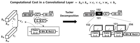
Figure 47. Tucker decomposition result of the first of the convolutional layers requiring computational reduction inside DUNET.

Figure 5. Operational workflow of eDenoizer.
3. Scheduling Framework for Multiple Deep Learning Models
As described in Figure 4, theour second objective is to keep ΔDi and ΔIi minimized while DUNET, the defense target model performing inference using the result of DUNET and various other deep learning models, are performed simultaneously with each other.
Once the system is started, the deep learning models to be performed are loaded from the system memory to the GPU memory. Please note that IoT edge devices use embedded GPUs. Furthermore, they do not have a separate dedicated memory and shares the system memory referenced by the CPU. Therefore, when deep learning models are loaded into GPU memory, data copy does not occur, and instead only memory location information (i.e., pointer) is delivered from the memory set on the CPU side [3][27].