1. The 4–20 mA Analogue Standard (Integration and Performance Improvement)
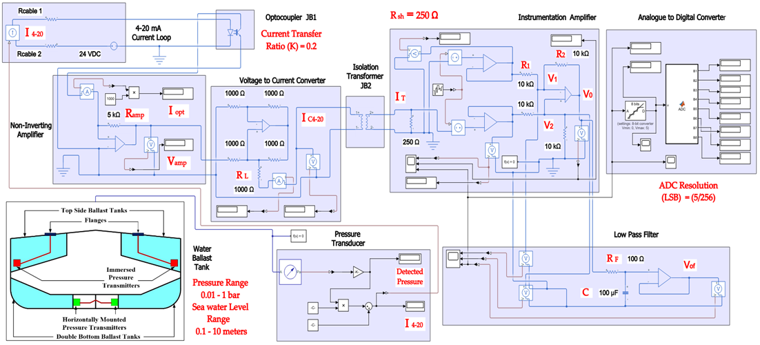
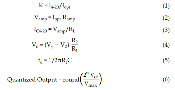
The 4–20 mA analogue standard is the most popular analogue standard used for the purpose of measurement and control in maritime automation and instrumentation fields. The non-zero lower range limit of 4 mA in addition to its high level of immunity to noise sources are the main reasons behind the popularity of the 4–20 mA analogue standard. The main principles of the 4–20 mA analogue measurement and control current loop were discussed in [2]. As previously discussed, the tank level measurement system is based on the use of classical 4–20 mA pressure transmitters to measure the fluid levels in the ships’ tanks. In order to provide more comprehensive realization for the 4–20 mA analogue standard, it should be analyzed as a part of the whole instrumentation or automation system [27 pp. 335–338]. Figure 3 illustrates a block diagram for a Simulink Simscape model (Figure 4) that describes how a single 4–20 mA pressure measurement current loop is integrated into an automation system. Based on the connection diagram in Figure 1, each pressure transmitter consists of a pressure sensor and a P/I transducer. A pressure sensor detects the applied pressure to its diaphragm, while a pressure transducer converts the detected pressure into a 4–20 mA analogue current signal proportional to a supposed pressure detected from 0.01 to 1 bar (range calibration). The 4–20 mA controlled current source [2] simulates the generated analogue current proportional to the applied pressure. Cable resistance is taken into account [2] in the described model. The measured 4–20 mA (I4-20) analogue current is applied to an optocoupler to perform the first stage of signal isolation [27 pp. 342–345,28] recommended at junction boxes (J.B1). Assuming that the expanded optocoupler model in [29] was adopted to provide galvanic isolation at (J.B1), the output current of the optocoupler (Iopt) will be decreased linearly from the input current by a current transfer ratio (K) of 0.2 using Equation (1). Therefore, additional signal conditioning circuitry is needed to restore the original measured 4–20 mA signal. This circuitry includes a non-inverting amplifier and a grounded load voltage-to-current converter [30,31]. The output voltage of the non-inverting amplifier (Vamp) calculated by Equation (2) will be converted to the current (IC4-20) through the load resistance (RL) in order to restore the original 4–20 mA measured current from this amplified voltage signal through Equation (3). After the 4–20 mA measured signal was restored at the location of the first junction box near the transmitter, it will continue to flow through the two-wires cable to the junction box near the control system (J.B2) where additional signal isolation will be applied through an isolation transformer (the Simscape ideal transformer block can be used to represent either an AC transformer or a solid-state DC-to-DC converter, and the two electrical networks connected to the primary and secondary windings must each have their own electrical reference). The output current of the isolation transformer (IT) is applied to the analogue input module in the control system where a 250 ohms shunt resistor (Rsh) will be used to convert the 4–20 mA current signal into a 1-5 VDC voltage signal. The converted voltage signal will be applied to an instrumentation amplifier [32] to eliminate any common mode noise voltage signals, as calculated in Equation (4). The instrumentation amplifier includes two buffer amplifiers and one difference amplifier. The buffer amplifier is used for signal transfer from the high impedance side to the low impedance side of the op-Amp [32]. The difference amplifier detects the difference between the applied voltage to both the non-inverting input (V1) and inverting input (V2) of the op-Amp, which leads to elimination of any similar in phase signals such as common mode voltages (Figure 5) induced by common mode noise (represented by a source of additive white Gaussian noise applied to the non-inverting inputs of the two buffers) [32]. The output voltage signal of the instrumentation amplifier is applied to an active low-pass filter [33] to eliminate high-frequency coupled noise to the measured signal (Figure 5). The cut-off frequency (fc) can be calculated using Equation (5). The analogue voltage output signal from the LPF (Vof) is converted to a digital signal through using an 8-bit analogue-to-digital converter, which consists of a quantizer
(quantized output is calculated through Equation (6) where n = 8 and Vmax = 5 VDC) and MATLAB-based function (Appendix A) to convert the detected output of the quantizer into 8 bits of binary data. The binary output of the analogue-to-digital converter can be transmitted to the CPU of the system controller through serial communication interfaces (RS 232 or RS485) or serial communication protocols such as Modbus RTU (relatively popular in maritime applications) [2].
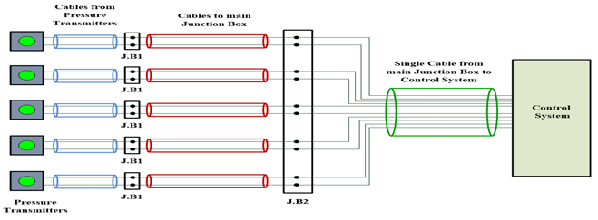
Figure 1. Connection diagram between 4-20 mA pressure transmitters and I/O modules in control system
Figure Int4. Simulink Simscape model used to simulate 4–20 mA pressure measurement current loop as a part of automation system.
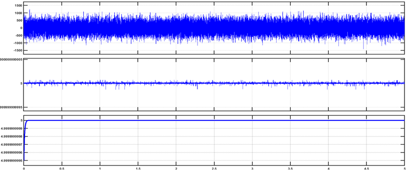
Figuroductione 5. Illustration of 5 VDC voltage signal corresponding to 20 mA analogue current (1 bar of detected pressure). Upper figure illustrates voltage signal highly distorted by common mode noise at difference amplifier input. Middle figure illustrates the output voltage signal of instrumentation amplifier slightly distorted by coupled noise, while the lower figure illustrates output voltage after low-pass filtering.
2. Foundation Fieldbus (Wired Digital Measurement and Control)
The Foundation Fieldbus protocol is a digital communication protocol adopted by many smart transmitters. The basic principles of the Foundation Fieldbus protocol were briefly discussed in [2,9,10] ([11], pp. 21–55) [12,13]. Foundation Fieldbus IEC 61,158 is a fieldbus protocol that basically counts on the idea of using a single twisted pair of wires for the connection of multiple field devices, the role of which will be extended beyond the regular role of measuring process variables to the role of performing automation and control tasks independently of the authority of the master controller. Field devices perform such tasks by using the feature of distributed data transfer (DDT) functions [2,9,10] ([11], pp. 21–55) [12,13]. Foundation Fieldbus also has the ability of providing a reliable measurement and control operations in explosive hazardous application areas depending on intrinsically safe models such as the entity model, FISCO model, FNICO model, HPTC model and DART model. Foundation Fieldbus is very similar to Profibus PA; however, Profibus PA is more popular in Europe while Foundation Fieldbus is more popular in Asia and America.
The Foundation Fieldbus signal is a Manchester-coded rectangular signal from the theoretical point of view; however, it is practically a trapezoidal waveform with rising and falling edges due to multiple factors such as delay imposed by modulation/demodulation electronic circuitry. The practical processing of a 31.250 Kbps Foundation Fieldbus Manchester-coded signal on the H1 bus was discussed in detail in [13], including modulation/demodulation techniques in noiseless as well as noisy conditions. The H1 bus is dedicated to the connection of all field devices along the same field bus; however, the HSE bus (high-speed ethernet) is dedicated to performing communication tasks between host controllers with a bit rate of 1–2.5 Mbps.
Foundation Fieldbus adopts a distributed communication system in which LAS (link active scheduler) plays an important role in controlling the communication [2,9,10] ([11], pp. 21–55) [12,13] process. For the purpose of redundancy, a single network may have two link masters, and in case one failed as the LAS, the other one will replace it. Communication between the LAS and field devices is divided into scheduled and unscheduled communication.
Foundation Fieldbus is one of the most popular digital communication protocols based on which smart sensors are built. Distributed Data Transfer (DTT) is the main principle according to which communication tasks in Foundation Fieldbus protocol are carried out. Like all communication protocols adopting fieldbus technology, Foundation Fieldbus allows for the connection of up to 32 field devices to a single twisted pair of wires in a single segment, provided that the field bus should be terminated from both sides in order to avoid jitter and reflections which might lead to communication failure. In Foundation Fieldbus protocol, the field devices can administrate some communication tasks regardless of the authority of the host controller. The communication process in Foundation Fieldbus protocol is supervised by the LAS (Link Active Scheduler) which can be any of the field devices connected to the fieldbus. Communication tasks in Foundation Fieldbus are divided into two categories, cyclic and acyclic tasks. Acyclic communication tasks take place at the time breaks between time intervals dedicated to cyclic communication. The type of data processed in cyclic communication is mainly related to process control and measurement variables, while the type of data processed in acyclic communication tasks is related to diagnostic and parametric information.
Unscheduled communication is used for the transaction of diagnostic data and field device parameters. It takes place during breaks between scheduled communication intervals. Scheduled communication can be divided into two categories: the first one is related to control and measurement variables, while the second one is related to system management [2,9,10] ([11], pp. 21–55) [12,13]. In the first category, a field device periodically publishes its process data to the entire fieldbus buffer directly upon receiving a compel data command (CD) from the LAS [10,12,14]. In the second category, each field device will receive independent schedules (time distributions (TD)) for data transaction.
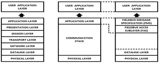
2.
As an OSI model (
Foigundation re 2
), Foundation Fieldbus is divided into three layers, which are the user application layer, communication stack and physical layer [9,10] ([11], pp. 21–55) [12]. The communication stack performs only the roles of data link layer and application layer. A Foundation Fieldbus management system consists of two layers: the first one is the application layer, which is included in the communication stack, and the second one is the user application layer, which consists of function blocks and device description. The application layer included in the communication stack consists of fieldbus message specification (FMS) and a fieldbus access sublayer (FAS) [9] ([11], pp. 21–55).
Figureldbus 2.
Foundation Fieldbus OSI (open systems interconnection) model.
Field devices can be easily connected to the bus during operation through using the probe node (PN) command [10,12] issued by the LAS to detect the newly connected field devices to the bus. The field device will be automatically assigned an address directly after it responds to the PN command with the probe response (PR) command. Afterwards, the LAS cyclically issues a pass token (PT) command in order to check if the field device is still functional or not by acknowledging the device response to the transmitted PT. If the device fails to respond for several times, it will be automatically excluded from the field devices’ live list.
The statistical process monitoring block (SPM) [15] can be considered one of the most important function blocks at Foundation Fieldbus smart transmitters. Its task is to construct a noise signature of the transmitter primary variable with both mean and standard deviation values. SPM enables the transmitter to detect any sudden changes that may be related to some physical disturbances, such as propagation or vibration (swaying or pitching on a ship, for instance), which are not reflecting an actual real-time measured value.
In a Rosemount 3051 FF smart pressure transmitter, the SPM block consists of three modules [15], which are:
-
Statistical calculation module: The measured pressure values are applied to high-pass filter to detect any slow changes, such as set point modifications, and eliminate them while constructing the input signal noise signature. The mean value is calculated for the unfiltered signal, and the standard deviation will be calculated over the filtered signal.
-
Learning module: responsible for establishing the process baseline values based on mean and standard deviation values calculated by the previous module.
-
Decision module: it compares the measured value with the baseline, to decide if an alert/alarm should be activated or such a measured value should be ignored.
3. Proposed Foundation Fieldbus (FF) Solution
The proposed solution is based on the replacement of classical 4–20 mA pressure transmitters used in the tank level measurement system on a bulk carrier commercial ship with Foundation Fieldbus pressure transmitters. Simulation models created by Emerson Segment Design Tool and Pepperl + Fuchs Segment Checker will simulate a safe area as well as explosive hazardous areas’ operational conditions. Therefore, the proposed solution will take into account possible non-intrinsically safe as well as intrinsically safe FF models, as follows:
- Non-intrinsically safe model.
- Intrinsically safe entity model.
- FNICO (Fieldbus Non-Incendive Concept) model.
- FISCO (Fieldbus Intrinsically Safe Concept) model.
- HPTC (High-Power Trunk Concept) model.
- DART (Dynamic Arc Recognition and Termination) model
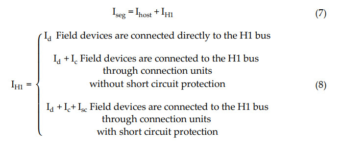
The recommended solution relies on replacement of the top side’s 10 immersed classical 4–20 mA transmitters with Foundation Fieldbus Rosemount 5400 non-contact radar transmitters and also replacement of the double bottom’s 14 classical 4–20 mA transmitters with Foundation Fieldbus Rosemount 3051 pressure transmitters. Each type of the previously mentioned models will be divided into two types of sub-models. The first one is for double bottom tanks, while the second one is for top side tanks. Each of these sub models consists of a single or multiple segments according to the requirements imposed by each sub-model. The total number of segments is determined according to the maximum allowable current withdrawn from the segment power supply. The total current consumption in a FF segment (Iseg) is the sum of current consumed by the host (Ihost) and the current consumed by the H1 bus (IH1) as indicated in Equation (7). The segment power supply should be able to withstand the sum of both currents. The maximum capacity of the segment power supply is dependent of the FF model adopted by the segment. For the non-intrinsically safe model, entity model, FISCO, FNICO, DART and HPTC (only when segment protectors are used) models, the current consumed by the H1 bus is simply the sum of the current consumed by all field devices (transmitters and actuators) if these devices were directly connected to the H1 bus without connection units such as megablocks; however, if those field devices were connected to the H1 bus through connection units, additional current will be consumed by these units. The current consumed by the connection unit is the sum of the operation current (Ic) and the current consumed by the field devices (Id) connected to the unit . In case the FF segment included connection units supporting short-circuit protection, Emerson Segment Design Tool calculates the short-circuit current (Isc) only once (near the segment terminator) at the last connection unit with short-circuit protection connected to the bus. The reason the short-circuit current is calculated only once along the H1 bus is that all field devices are connected in parallel to the same field bus, so in case a short circuit occurred, the whole H1 bus will suffer a failure.
Unlike FISCO and FNICO models, the High-Power Trunk Concept does not impose any limitations on the maximum available power at the Fieldbus trunk cable, which allows for longer cable lengths and a higher number of field devices per segment. The High-Power Trunk Concept allows for an output voltage up to 30 VDC and a maximum current up to 500 mA. The basic idea of a High-Power Trunk Concept is to provide unlimited energy to the field bus trunk; however, within the hazardous area, this unlimited energy will be distributed using energy-limiting wiring interfaces till it is delivered to the field device. HPTC does not require power supply conditioners particularly dedicated to the model, as standard non-intrinsically safe lower price power supplies can be used in the HPTC network. Energy-limiting wiring interfaces include field barriers and segment protectors. They both provide short-circuit protection as well as galvanically isolated outputs [11] (pp. 114–129) [34,35,41]. Each of these outputs acts as a FISCO or entity power supply. HPTC allows for a maximum number of four field barriers. Each of these barriers allows for up to four field devices. Therefore, HPTC allows for up to 16 field devices per segment. According to the simulation results that will be discussed later, there are two major differences between segment protectors and field barriers. The first difference is related to the available voltage at the output terminals to which field devices are connected. Segment protectors maintain constant voltage at a specific field device connected to a specific segment protector regardless of the voltage drop on the spur. Field barriers maintain constant output voltage all along the segment at the output port dedicated to a specific field device regardless of the total voltage drop on the H1 bus main trunk cable. Segment protectors are used with Zone2/Div2 applications; however, field barriers are used with Zone1/Div2 applications. Therefore, the voltage available at field barrier output terminals connected for field devices is less than the voltage available at segment protector output terminals for field devices, as will be shown in the simulation results. The second difference between segment protectors and field barriers, which was observed during simulation, is that the value of the current consumed by each field barrier is dependent of the following variants:
- The total current of field devices connected to the field barrier (IdT).
- The H1 bus main trunk overall cable length (LT).
- Number of field barriers included in the segment (NFB) and current consumed by each of them (IdTS).
- Length of H1 bus main trunk cable sections between field barriers (LFB).

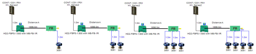
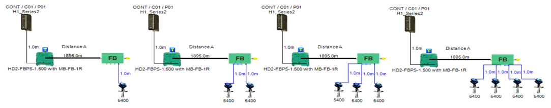
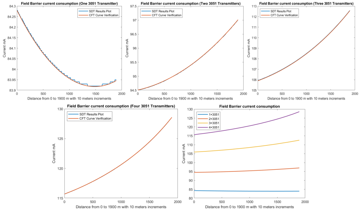
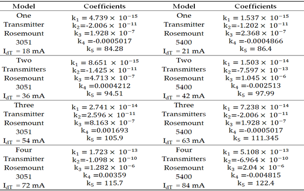
In order to define the characteristics of the relation between some of the previously mentioned variants and the current consumed by the field barrier, simple HPTC segments (Figure 6) were constructed using Emerson Segment Design Tool to derive the relation between the first two variants (IdT and LT) and the current consumed by the field barrier. Four of these segments are dedicated to Rosemount 3051 transmitters (Figure 6a), while the other four segments are dedicated to Rosemount 5400 transmitters (Figure 6b). In each of these segments, the current consumed by field barriers will be calculated with respect to the change in the distance A between the field barrier and the power supply from 10 m to 1895 m, with increments of 10 m. These calculations will be performed when one, two, three or four transmitters are connected to the field barrier. Results of these simulation models were plotted using MATLAB. Curve Fitting Tool in MATLAB was used to derive the mathematical equations describing the obtained simulation plots for each of the models in Figure 6. The mathematical equations obtained were verified by the same MATLAB code providing curves similar or identical to the simulation plots. These mathematical equations characterized the relation between field barriers’ current consumption and length of H1 bus cable (for a specific number of field devices connected to the barrier) as a polynomial relation of the fourth degree. This polynomial relation is generally described in Equation (10) where (IFB) is the current consumed by the field barrier, and (LT) is the length of the H1 bus cable between the power supply and field barrier. The values of coefficients k1, k2, k3, k4 and k5 are used to distinguish between the eight models illustrated in Figure 6a,b. The values of these coefficients for each of these eight models are indicated in Table 2. Figures 13 and 14 both illustrate the SDT (Segment Design Tool) simulation plots as well as the equation verifying curves for the models illustrated in Figure 6a,b, respectively. It would be worth mentioning that the obtained equations are applicable only for the models illustrated in Figure 6, which means that for another segment structure, where more field barriers as well as more field devices are added, the current consumed by the field barriers will be dependent of not only IdT and LT (similarly to segments in Figure 6) but also dependent of IdT, NFB and LFB.
6(a)
Each Foundation Fieldbus segment should include a segment power supply the capacity of which is dependent on the Foundation Fieldbus model adopted by the segment. Other than regular power supplies, FF segment power supply ensure impedance matching all along the bus, in addition to superimposing the Manchester coded signal rendered by the host on the supply voltage (9-32 VDC) provided to the field devices included in the segment. The model (Non-intrinsically safe/intrinsically safe) adopted by an FF segment is basically determined by the safety requirements imposed by the location at which the field devices included in the segment will be installed. For safe-area applications, non-intrinsically safe model will be adopted while for explosive hazardous areas, an intrinsically safe model will be adopted. Foundation Fieldbus allows for up to 5 intrinsically safe models:
1-Entity model.
6(b)
2- FISCO (Fieldbus Intrinsically Safe Concept) model.
Figure 6. Test segments (a,b) dedicated to deriving the relation between main FF trunk cable length and current consumed by field barriers. (a) Test segments using Rosemount 3051 Pressure Transmitters; (b) Test segments using Rosemount 5400 Radar Transmitters.
3- FNICO (Fieldbus Non-Incendive Concept) model.
4- HPTC (High-Power Trunk Concept) model.
Figure 13. Illustration of current consumed by field barrier with respect to FF H1 trunk cable length when for four models in which one, two, three or four 3051 transmitters were connected to the field barriers in the models in Figure 6a.
5- DART (Dynamic Arc Recognition and Termination) model.

Entity model allows for a segment power supply capacity of 80 mA, which makes it possible to connect 2-3 field devices per segment. According to Entity model, cable characteristics (Resistance, inductance and capacitance) are taken into account during ignition curves estimation, that's why, more restrictive curves (inductive curves) are considered in intrinsically safe calculations. Other than Entity model and based on experimental results, FISCO model neglects cable characteristics during intrinsically safe calculations which allows for segment power supply capacities of 320 mA and 180 mA for IIB and IIC applications respectively. FNICO model is an extension for FISCO model, however FISCO model is dedicated to Zone1/Division 1 applications, while FNICO model is dedicated to Zone2/Division 2 applications. The main idea of any intrinsically safe system is to limit the energy that might lead to ignition in explosive hazardous areas. Both of Entity and FISCO models are undertaking such a mission by limiting the energy level all along the segment (cables, connection units and output ports). Other than Entity and FISCO models, HPTC model limits the energy in explosive hazardous areas only at connection interfaces (segment protectors or field barriers) to which field devices are connected. In other words, HPTC model distributes the energy consumed by the segment all along the segment so that minimal levels of energy can be ensured at field devices installed at explosive hazardous areas through using dedicated connection interfaces to provide reduced level of energy for such devices. There are two types of connection interfaces adopted by HPTC model, segment protectors and field barriers. Segment protectors are used for Zone2/Division2 applications, while field barriers are used for Zone1/Division 1 applications. Two major differences distinguish between segment protectors and field barriers. Firstly, segment protectors maintain constant voltage at a specific field device connected to a specific segment protector regardless of the voltage drop on the spur, while field barriers maintain constant output voltage all along the segment at the output port dedicated to a specific field device regardless of the total voltage drop on the H1 bus main trunk cable. Secondly, the current consumed by segment protector is simply the sum of the operating current of the segment protector (4-5 mA) in addition to the sum of the currents of all field devices connected to the segment protector and the assumed short circuit current, however for field barriers the overall current consumed by the barrier is determined by five variants indicating the mechanism by which HPTC model performs the role of limiting the energy in specific locations all along the segment (locations where field devices are connected to the bus through field barriers). In case it was assumed that a single FF segment adopting HPTC model included multiple field barriers to which a number of field devices are connected, the current consumed by each of these field barriers will be dependent on the following variants:
1- The overall length of the H1 bus trunk cable.
For all FF models except for the HPTC model, voltage drop at any field device in the segment can be calculated by Equation (11) where Vsupply is the available voltage from the segment power supply, VH1 is the voltage drop on the H1 bus main trunk cable from the power supply to the device, Vc is the voltage drop on the connection unit to which the field device spur is connected and Vspur is the voltage drop on the spur to which the field device is connected. For all connection units (megablocks, segment protectors and field barriers), there is no voltage difference between input and output terminals connected to the H1 bus main trunk cable. VH1 is dependent of the total current consumption in the segment and overall length of the main H1 bus trunk cable, while Vspur is dependent of spur length and field device current connected to the spur. The voltage drop on any connection unit Vc exists between the input terminals connected to the H1 bus main trunk cable and the output terminals dedicated to spur connections. In the simulated models, Vc was equal to zero in all models except for the HPTC model based on using field barriers and segment protectors. In the DART model, Vsupply will be decreased only in the first 5–10 microseconds of possible spark ignition in order to reduce the voltage delivered to the field device so that the spark would be early extinguished.
2- The lengths of the cable sections connecting between the field barriers.

3- The current consumed by the field barriers which precede and follow that specific field barrier
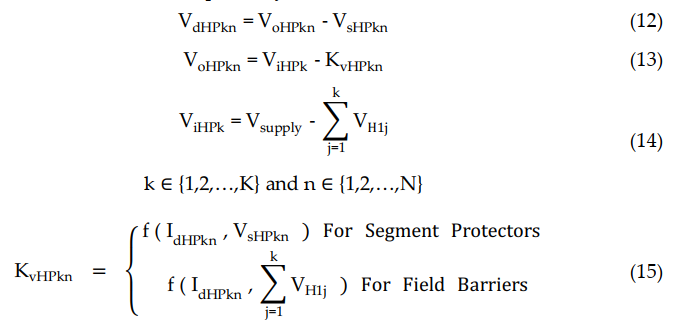
In HPTC sub-models with the segment protectors HPTC-SP-TS and HPTC-SP-DB, constant voltage was maintained at field devices, irrespective of the voltage drop on the spur. When increasing the spur length to which the field device is connected, the segment protector will increase the voltage at the output terminals to compensate the increased voltage drop on the spur. The output voltage of the segment protector is decreased from the segment protector input voltage by a reduction coefficient, the value of which for a specific field device will decrease when increasing the spur length. In HPTC sub-models with the field barriers HPTC-FB-TS and HPTC-FB-DB, output ports dedicated to connecting field devices of a specific current maintained constant voltage all along the segment, irrespective of the voltage drop on the H1 bus trunk main cable. This constant output voltage is maintained through compensating the decreased input voltage at farther field barriers by a reduction coefficient, which is decreasing from the nearest field barrier to the farthest field barrier in the segment. For an HPTC segment consisting of K connection units (field barriers or segment protectors), each (k) connection unit has N output ports for connecting field devices. For a field device (n) connected to the connection unit (k), the voltage level at the field device (VdHPkn) will be the difference between output voltage form the connection unit at the port connected to the device (VoHPkn) and the voltage drop on the spur to which the device is connected (VsHPkn). The input voltage to the (k) connection unit (ViHPk) is reduced by a reduction coefficient (KvHPkn) the value of which is dependent on the type of the connection unit, whether it was a field barrier or a segment protector. If the connection unit was a segment protector, the value of the reduction coefficient will be a function of the field device current (IdHPkn) and voltage drop on the spur to which the field device is connected. If the connection unit was a field barrier, the value of the reduction coefficient will be a function of the field device current and the sum of the voltage drops on the H1 bus main trunk cable from the power supply to the field barrier.
4- The overall current consumed by the field devices connected to that specific field barrier.
5- The total number of field barriers included in the segment.
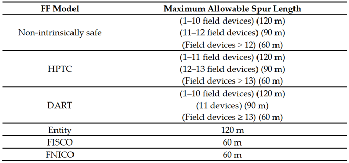
According to the simulation results obtained from Emerson Segment Design Tool, Table 3 illustrates the maximum allowable spur lengths in different Foundation Fieldbus models. For non-intrinsically safe, HPTC and DART models, maximum allowable spur length is dependent on the total number of field devices per segment; however, for entity, FISCO and FNICO models, the maximum allowable spur length in the segment is a constant value independent of the total number of field devices per segment.
The results obtained from simulation of Foundation Fieldbus HPTC test segments constructed by Emerson Segment Design Tool were analyzed using MATLAB to derive the mathematical equation describing the polynomial relation between the current consumed by the field barrier and the overall length of H1 bus main trunk cable (excluding the lengths of the spurs) for specific total current consumption by the field devices connected to the barrier. Due to such a polynomial relation, It was noticed that the current consumed by the field barrier tends to increase when increasing the length of the total H1 bus trunk cable. The rate of such a current increase is proportional to the total consumed by the field devices connected to the barrier. Moreover and due to the technique adopted by HPTC model to distribute the segment energy all along the segment, the overall noticed current consumption in an FF HPTC segment using field barriers, is the highest in comparison with the overall current consumption if other FF models were adopted (Non-intrinsically safe, Entity, FISCO, FNICO and DART). DART model is the latest intrinsically safe model adopted by Foundation Fieldbus protocol. The basic idea of DART model is to extinguish the spark at an early stage of its formation based on the calculated current rate of change with respect to time. This process is administrated by dedicated segment power supply the capacity of which is 360 mA. The segment power supply limits the energy of the bus only at the first 5-10 microseconds of spark ignition so that it can be early extinguished.