Your browser does not fully support modern features. Please upgrade for a smoother experience.
Please note this is a comparison between Version 2 by Vivi Li and Version 1 by Ataur Rahman.
Flood is one of the most destructive natural disasters, causing significant economic damage and loss of lives. Numerous methods have been introduced to estimate design floods, which include linear and non-linear techniques. Since flood generation is a non-linear process, the use of linear techniques has inherent weaknesses. To overcome these, artificial intelligence (AI)-based non-linear regional flood frequency analysis (RFFA) techniques have been introduced over the last two decades.
- regional flood frequency analysis
- artificial neural networks
- flood
- artificial intelligence
1. Introduction
Flood is one of most devastating natural disasters, resulting in significant economic losses including human deaths [1,2][1][2]. This damages both rural and urban infrastructure like bridge and drainage systems [3,4][3][4]. Flood generally leaves undesirable sediments and debris in the affected lands [5[5][6],6], which can disrupt transportation networks [7], clog drainage infrastructure and sewers [8,9][8][9] and may make lands unproductive. The cleaning up of flood debris is usually costly, not to mention the disruption to the daily lives of the community involved [10,11][10][11]. Due to climate change, the frequency and magnitude of floods are increasing [12].
Flood forecasting requires significant efforts, and it is usually the responsibility of a large government organisation. Governments spend a significant amount on various projects to identify flood-safe areas, which are used to build cities. Researchers have developed numerous methods to estimate design floods, which are used to build flood-safe infrastructure [13,14][13][14]. Design flood is defined as a flood level or discharge associated with a return period or annual exceedance probability such as a 100-year flood.
In addition to traditional techniques, like the rational method, physical and numerical [15,16][15][16] models have been proposed for design flood estimation. Most of the physical models require in-depth knowledge of flood processes [17[17][18],18], making them difficult to use in practice. Van den Honert and McAneney [19] pointed out the common limitations associated with these physical models [20[20][21],21], which include model inaccuracies resulting in systematic errors (over or underestimation of design floods) [22,23][22][23]. On the other hand, data-driven models have been quite popular for flood estimation in recent years [24]. Examples include a quantile regression technique and a probabilistic rational method [25]. This is because they usually consider climate factors and catchment characteristics in developing models, which are easier to apply [26,27][26][27]. A flood frequency analysis (FFA) is the most popular method to estimate design floods, which uses observed peak discharge data disregarding catchment characteristics [28,29][28][29]. A normal distribution [30[30][31],31], log-normal distribution [32[32][33],33], Gumbel distribution [34[34][35],35], generalised extreme value distribution and log-Pearson type III distribution [36,37][36][37] are some of the most commonly used flood frequency distributions in FFA. One of the major limitations of FFA is the lack of long and good quality recorded flood data at the location of interest. To overcome data limitations, hydrologists have proposed a regional flood frequency analysis (RFFA), which attempts to estimate design floods at an ungauged catchment based on the concept of a homogeneous region, which pools observed flood data from a group of similar catchments to estimate design floods at the ungauged catchment [38,39][38][39]. This method became more popular among researchers than physical models because it saves time and resources [40]. Probabilistic rational method (PRM) [41], multiple linear regression (MLR) [42,43][42][43], quantile regression techniques (QRT) [44[44][45],45], and index flood method (IFM) [46,47][46][47] are some of the most commonly used RFFA techniques. However, some of the early RFFA techniques (e.g., rational method) have lost their popularity due to their inconsistency and inappropriate model assumptions.
In the past two decades, scientists suggested hybrid or mixed methods to increase the relative accuracy of RFFA models [48,49][48][49]. Although some early linear models have been improved, they may not be accurate under some circumstances as flood generation is basically a non-linear process [50]. Hydrologists attempted to apply non-linear methods in RFFA such as a non-linear regression analysis (where log-transformation of the variables is considered). Artificial intelligence (AI)-based methods are also non-linear, but more powerful than simple non-linear models like log-log ones as they can consider many different combinations of variables and complex non-linear processes in model building. Given that the majority of flood estimation methods are data driven, they require a great deal of simplification and assumptions to be practical, accessible, and implementable [51,52][51][52]. They require relatively fewer input data and minimal knowledge of fundamental physical processes involved. Over the last two decades, non-linear AI-based RFFA methods have grown in popularity over physical models as these provide more accurate results and are easier to apply [53,54][53][54]. Artificial neural networks (ANNs) [55,56][55][56], support vector regression (SVR) [57[57][58][59][60],58,59,60], adaptive neuro-fuzzy inference system (ANFIS) [61[61][62],62], genetic algorithms (GA) [63,64][63][64] and hybrid, mixed and combined approaches [65,66][65][66] are some of the most popular AI-based flood estimation methods. As AI-based models are relatively new in flood estimation, it is not easy to decide which one is to be applied for a given problem [67,68][67][68].
There are several important aspects to consider when building models based on AI. Firstly, these models like all other data-driven models need enough data to develop and test the model [67]. If adequate data exist, it is often possible to build, test, and evaluate an AI-based model (similar to many other RFFA models) by dividing the data into training, test, and evaluation data sub-sets [69,70][69][70]. Cross-validation is also often used in building RFFA models when less data samples are available [71]. The more data used in the modeling, the less generalization error occurs, meaning that the final model can be used on different sites with limited or no data available. Other benefits of having adequate data include the simplicity of using different distribution methods, the ability to account for lost data or missing variables, and, most crucially, the ability to train and validate the model multiple times to develop the best possible model [72,73][72][73]. However, it should be noted that data quality is of significant importance in developing and testing accurate models.
2. AI-Based RFFA Methods
Figure 21 illustrates how to develop an AI-based RFFA model. It is important to identify input variables. Some of the most used input variables include catchment area (A), longitude (LON), latitude (LAT), elevation (EV), drainage density (DD), average annual maximum daily precipitation (AP), rainfall intensity (I), vegetation coverage (VC), slope (SL), and relative elevation (RE), fraction forested area (F), mean annual evapotranspiration (MAE), shape factor (SF), and stream density (SDEN). Output variables include maximum stream flow, flood quantiles, and time to peak. Collected data are then standardised to avoid a scaling problem. To build a reliable model, training, validation [69[69][70],70], and test data are required. Different statistical measures are used to compare alternative models such as RMSE, RMSNE, and R2.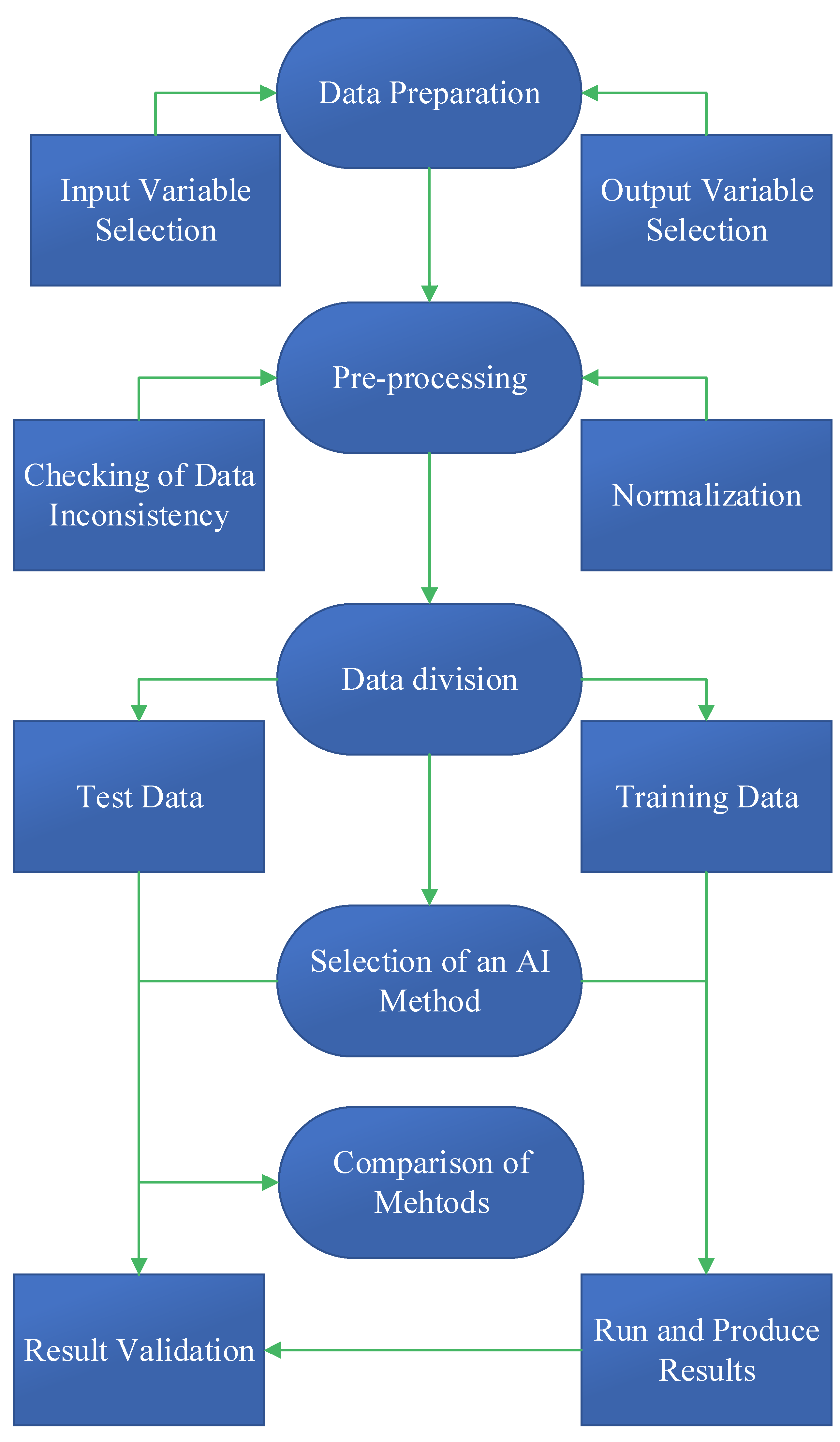
Figure 21.
Steps in building an AI-based RFFA model.
2.1. ANN-Based RFFA Models
The ANN performs like a human nervous system in that it learns from previous trials and decides how to come up with a better model by exploiting the best possible links between dependent (flood quantiles such as Q10) and independent variables (such as rainfall) in a series of steps. ANN, as a data-driven tool, does not require any physical knowledge of flood processes involved [78,79][74][75]. One of the limitations of this method is lack of physical interpretation of the developed models. Shu and Burn [51] compared the ANN with a parametric regression analysis in one of the first articles on the AI-based RFFA. They found that a properly developed ANN model outperforms both linear (REG-OLS) and non-linear (REG-NONLINEAR) regression-based methods. They also compared the results of a single ANN to those of ANN ensembles, concluding that the latter provided more accurate flood estimates. Jingyi and Hall [80][76] compared four different models, including the residuals method, Ward’s method, fuzzy c-mean, and a variation of the ANN, known as the Kohonen network. They found that, while other methods may be somewhat useful, the ANN method produced the lowest standard error of estimate and could be a useful method if adequate data from enough sites are available. Dawson et al. [81][77] applied ANN using data from 850 stations. They compared the results of the ANN method to those of multiple regression models and found that ANN outperformed the other models. They noted that because there is little need to understand the physics of flood generation processes, scientists from all disciplines, not just hydrologists, could use the ANN method. Shu and Ouarda [56] developed RFFA models based on ANN and CCA using data from 151 catchments and found that the ANN–CCA combination provided better generalisation and accuracy. Srinivas et al. [49] used AI-based RFFA and regression methods involving various AI-based algorithms. To determine the best approach for data clustering, a regression analysis, CCA, and FCM algorithms were compared. They found that leave-one-out cross-validation based on the FCM algorithm produced better results when evaluating the accuracy of the estimated flood quantities.2.3. SVM-Based RFFA Models
The SVM method is widely used for classification, which examines data at higher dimensions [107,108][78][79]. Several types of kernels assist SVM in classifying data by minimising data margins, eliminating outliers, and focusing on relationships between the test and training data. The most common kernel types used for developing SVM-based models include linear, polynomial, radial basis function (RBF), and sigmoid function. Among these, the SVM-based RBF kernel is the most used method that produces robust and consistent results. Gizaw and Gan [109][80] developed RFFA-based ANN and SVR methods using data collected from 49 stations in Canada. When the results of these two methods were compared, they found that the SVR method outperformed the ANN in terms of consistency and generalisation ability. They also mentioned that better SVR performance could be attributed to smaller datasets, whereas ANN would most likely produce more accurate results for larger datasets. Sharifi Garmdareh et al. [110][81] estimated design floods using SVR, ANFIS, ANN, and NLR methods using more than 20 years of recorded data from 55 hydrometric stations in Iran. They tested various strategies for determining the best combination of input variables and found that gamma testing (GT) was the most effective, which can improve the result of ANFIS and SVR over a single method and that using GT reduced the number of input variables. They also noted that combining GT with the ANFIS produced the best results, followed by GT + SVR. Ghaderi et al. [111][82] used ANFIS, SVM, and GEP to estimate flood quantiles with a 50-year return period. From 21 years of data collected from 47 catchments in Iran, they used GM and M-test to identify the most important predictor variables and the best ratio of test and training data. They compared the results of the three methods and noted that all three were “good” in terms of NASH, with the SVM method slightly outperforming the others in terms of R2 and RMSE. Vafakhah and Bozchaloei [112][83] used SVR, ANN, and NLR to estimate design floods using data collected from 33 stations in Iran over 20 years. They noted that, according to RRMSE and NASH, SVR is the most efficient method of the three and can be used for regional flood duration curve analysis. Haddad and Rahman [65] used 25 to 82 years of data from 202 catchments in Australia to evaluate 15 different combinations of multidimensional scaling (MDS), bayesian generalised least squares (BGLSR), and SVR methods to estimate design floods. They found that the MDS-based SVR method with RBF kernel outperforming others, including linear, polynomial, RBF, and sigmoid kernels, in terms of consistency and accuracy of the results. They also noted that using MDS improved the overall performance of all the methods. Allahbakhshian-Farsani et al. [59] used 19 years of data from 54 hydrometric stations in Iran to compare the performance of several AI-based RFFA methods. This sentudry employed methods such as SVR, multivariate adaptive regression spline (MARS), boosted regression trees (BRT), and projection pursuit regression (PPR). Using various statistical indices such as NASH, RMSE, RMSE, and R2, they noted that the SVR model based on the RBF kernel outperformed all the others, including non-linear regression. From the above discussion it can be stated that both SVM and SVR were used in RFFA. A large set of catchments are needed to group them into homogeneous sub-sets which can then be subjected to SVR to estimate flood quantiles.2.4. GA and Hybrid Type of AI-Based RFFA Models
Hybrid models typically produce better results. As shown in Table 1, many scientists have conducted experiments based on combining various AI-based RFFA models. Some of the most common hybrid models include genetic algorithm (GA) combined with ANN or ANFIS. The GA is commonly used as a hybrid method in conjunction with other methods, particularly ANN [106][84]. Another popular hybridisation technique used in RFFA is the combination of canonical correlation analysis (CCA) with ANN and ANN ensembles, as well as ANFIS methods. CCA improves the performance and reduces the complexity of ANN-based RFFA models by exploiting regional flood data [92,97][85][86].Table 1. Summary of AI-based RFFA studies (* indicates the best model) (ANN = Artificial neural network; GA = Genetic algorithm, BGLS-QRT-ROI: Bayesian generalized least squares QRT combined with region of influence approach, BNN = Backpropagation neural network, CANFIS = Co-active neuro fuzzy inference system, GEP = Gene-expression programming, GRNN = generalized regression neural networks, LGP = Linear genetic programming (LGP), LR = Linear regression, M5 = M5 model tree, MLP = Multi-layer perceptrons, MLR = Multiple linear regression, MNLR = Multiple non-linear regression, QRT = Quantile regression technique, RBNN = Radial basis function-based neural networks, G-EANN = generalized ANN-Ensembles, EANN = ANN-Ensembles, GAANN = GA-based ANN, BPANN = Back propagation for ANN, FIS = Fuzzy inference system, CCA = canonical correlation analysis, NLCCA = Non-linear canonical correlation analysis, BGLSR = Bayesian generalised least squares, MDS = multidimensional scaling, MARS = multivariate adaptive regression spline, BRT = boosted regression trees, PPR = projection pursuit regression, WNN = wavelet neural network and RFR = random forest regression).
| Reference | Author, Year | Model | Predictor Variables (Inputs) |
Model Output | Catchment, Year |
Journal | Country (Catchment) | RMSE * | RRMSE/NASH * | R2 * |
|---|---|---|---|---|---|---|---|---|---|---|
| [102][87] | Zalnezhad et al., 2022 | ANFIS(FCM) * ANFIS(SC) ANFIS(GP) QRT |
A, I, MAR, SF, MAE, SDEN, S1085, FOR | Q2–100 | 181 Stations 40–89 Year |
Water | Australia | 50.88 | RRMSE = 0.78 | NA |
| [97][86] | Desai and Ouarda, 2021 | CCA-RFR * PFR CCA-GAM EANN ANN CCA-MLR CCA-Kriging CCA-EANN CCA-ANN |
A, MBS, FAL, AMP, AMD | Q10–100 | 151 stations, ≥15 year | Journal of Hydrology | Canada (Quebec) |
0.05 | NASH = 0.57 RRMSE = 29.44 |
NA |
| [96][88] | Linh et al., 2021 | WNN * ANN |
SLP, SST | Max monthly discharge (MAD) | 3 stations, 37 years |
Acta Geophysica | Iran (Golestan Dam, Madarsoo) |
0.68 | NASH = 0.99 | 0.99 |
| [59] | Allahbakhshian-Farsani et al., 2020 | SVR * MARS BRT PPR NLR |
A, AA, AMP, MXP, NDP, CC, CR, TC, P, SL, DD, SS, MBS, PF, SDT, RA, BL, FLA, FOR, RLA, DA, WA, EL, MXEL, MNEL | Q2–200 | 54 stations, 19 years |
Water Resources Management | Iran (Karun and Karkhe River) |
50.70 | NASH = 0.94 RRMSE = 63.93 | 0.96 |
| [95][89] | Kordrostami et al., 2020 | ANN | A, AEV, AMP, FOR, I, SS, SF and DD | Q5–100 | 88 stations, 25–82 years |
Geosciences | Australia (New South Wales) |
NA | RRMSE = 0.48 | 0.74 |
| [65] | Haddad and Rahman, 2020 | MDS-SVR * MDS-BGLSR |
A, AEV, SF, DD, SS, FOR, I and AMP | Q2–100 | 202 stations, 25–82 years |
Natural Hazards | Australia (New South Wales and Victoria) |
NA | RRMSE = 56 | 0.78 |
| [112][83] | Vafakhah and Khosrobeigi Bozchaloei, 2020 | SVR * ANN NLR |
A, AA, AEV, P, MBS, MXEL, MNEL, EL, SL, DD, SS, AMP, T, PF, RLA, BL, GA, RA | Q2–90 | 33 Stations, 20 years | Water Resources Management | Iran (Namak Lake) |
0.11 | NASH = 0.91 RRMSE = 1.45 |
0.96 |
| [111][82] | Ghaderi et al., 2019 | SVM * ANFIS GEP |
A, P, MBS, EL, L, SL, SS, DD, MXSO, FF, L, CR, CC, AMP, MXP, BL, FOR | Q50 | 47 stations, 21 years |
Arabian Journal of Geosciences | Iran (South-west) |
239.94 | NASH = 0.75 | 0.76 |
| [110][81] | Sharifi Garmdareh et al., 2018 | ANFIS * SVR ANN NLR |
A, AEV, P, DD, MXEL, MNEL, MBS, EL, SL, SS, T, AMP, | Q2–100 | 55 stations, 20 years | Hydrological Sciences Journal | Iran (Namak Lake) |
8.40 | NASH = 0.90 | 0.95 |
| [67] | Aziz et al., 2017 | ANN * GEP * QRT |
A, AEV, AMP, SS, I | Q2–100 | 452 stations, 25–75 years | Stochastic Environmental Research and Risk Assessment | Australia (New South Wales, Victoria, Queensland and Tasmania) |
Na | NASH for ANN for smaller ARIs = 0.78 NASH for GEP for larger ARIs = 0.73 |
NA |
| [92][85] | Ouali et al., 2017 | NLCCA-GAM * NLCCA-EANN CCA-ANN CCA-EANN NLCCA-ANN NLCCA-GAM/ STPW |
A, MBS, FAL, AMP, AMD | Q10–100 | 151, 204 and 69 stations, ≥15 years | Journal of Advances in Modeling Earth Systems | Canada and United states (Quebec, Arkansas, Texas) |
NA | RRMSE = 0.28 NASH > 0.8 |
NA |
| [109][80] | Gizaw and Gan, 2016 | SVR * ANN |
A, SS, SL, TC, I, AMP | Q10–100 | 26 and 23 stations, ≥15 years |
Journal of Hydrology | Canada (British Columbia, Ontario) |
46.2 | NA | 0.7 |
| [106][84] | Aziz et al., 2016 | ANN * GAANN CANFIS GEP |
A, AEV, I, AMP, SS, | Q2–100 | 452 Stations, 25–75 years |
Artificial Neural Network Modelling (Book) | Australia (New South Wales, Victoria, Queensland and Tasmania) |
NA | NASH = 0.69 | NA |
| [61] | Kumar et al., 2015 | FIS * ANN L-moments (PE3) |
A, AMP, SDT, EL | Q2–1000 | 17 stations, 15–29 years | Water Resources Management | India (Godavari river) |
2.32 | Na | NA |
| [114][90] | Aziz et al., 2015 | GAANN BPANN |
A, I | Q2–100 | 452 stations, 25–75 years | Natural Hazards | Australia (New South Wales, Victoria, Queensland, and Tasmania) |
NA | NA | NA |
| [105][91] | Bozchaloei and Vafakhah, 2015 | ANFIS * ANN NLR |
A, AA, AEV, P, MBS, MXEL, MNEL, EL, SL, DD, SS, AMP, T, PF, RLA, BL, GA, RA | Q2–92 | 33 stations, 20 years | Journal of Hydrologic Engineering | Iran (Namak Lake) |
0.008 | NASH = 0.92 | 0.99 |
| [87][92] | Durocher et al., 2015 | PPR * | A, SL, SS, MBS, FOR, FAL, AMP, AMPS, AMPL, MLS, AMD | Q10–100 | 151 stations, ≥15 years | Journal of Hydrometeorology | Canada (Quebec) |
NA | RRMSE = 0.40 | NA |
| [86][93] | Alobaidi et al., 2015 | G-EANN * EANN |
A, MBS, FAL, AMD, AMP | Q10–100 | 151 stations, ≥15 years | Advances in Water Resources | Canada (Quebec) |
NA | RRMSE = 0.34 | NA |
| [85][94] | Aziz et al., 2014 | ANN * QRT |
A, AEV, AMP, SS, I | Q2–100 | 452 stations, 25–75 years | Stochastic Environmental Research and Risk Assessment | Australia (New South Wales, Victoria, Queensland, Tasmania) |
NA | NA | NA |
| [103][95] | Aziz et al., 2013 | BGLS-QRT-ROI * CANFIS | A and I | Q2–100 | 452 stations, 25–75 years |
Journal of Hydrological Environment Resources | Australia (New South Wales, Victoria, Queensland, and Tasmania) |
NA | NA | NA |
| [84][96] | Seckin et al., 2013 | MLP * L-moment RBNN GRNN MLR MNLR |
A, EL, LAT, LON, and RP | Q1.111–1000 | 13 stations, 10-39 years | Water Resources Management | Turkey (East Mediterranean River) |
0.173 | NA | 0.84 |
| [113][97] | Seckin and Guven, 2012 | GEP * LGP LR |
A, EL, LAT, LON, and RP | Q25.7–174.3 | 543 stations, ≥15 years |
Water Resource Management | Turkey (Rivers across the country) |
NA | NA | 0.57 |
| [83][98] | Singh et al., 2010 | BNN * M5 |
A, MRD, AMP, RP, MBS and FOR | Q2.33 | 93 stations, 10–83 years | Water Resources Management | India (Catchments across the country) |
NA | NA | NA |
| [82][99] | Ouarda and Shu, 2009 | ANN * Multiple regression model |
A, FAL, FOR, AMD, AMPL, NT27, CN | Q2–10 | 134 stations, ≥10 years | Water Resources Research | Canada (Quebec) |
27.33 | NASH = 0.96, RRMSE = 36.17 | NA |
| [55] | Shu and Ouarda, 2008 | ANFIS * ANN NLR NLR-R |
A, MBS, FAL, AMP, AMD, HDB, TOPO | Q10–100 | 151 stations- ≥15 years | Journal of Hydrology | Canada (Quebec) | 316 | NASH = 0.85 RRMSE = 57 |
NA |
| [49] | Srinivas et al., 2008 | SOFM * CCA Regional regression |
A, SS, SRC, SSC, AMP, SL, EL, FOR, R24h | Q2–100 | 11 stations, 6–42 years |
Journal of Hydrology | United states (Indiana) |
NA | RRMSE = 0.276 | NA |
| [56] | Shu and Ouarda, 2007 | ANN * ANN-CCA |
A, AMD, AMP, FAL, MBS | Q10–50 | 151 stations, ≥15 year |
Water Resources Research | Canada (Quebec) |
0.053 | NASH = 0.82 RRMSE = 38 |
NA |
| [81][77] | Dawson et al., 2006 | ANN * MLR |
A, AMP, L, DA, IF | Q10, 20, 30 | 850 stations, 20 years |
Journal of Hydrology | United kingdom (Catchment across the UK) |
NA | NA | NA |
| [80][76] | Jingyi and Hall, 2004 | ANN * Cluster analysis |
A, AMP, MXP, SL, SS, EL, GFI and PLN | Q50 | 86 stations 15–36 years |
Journal of Hydrology | China (Jiangxi and Fujian, Gan and Ming rivers) |
47 | NA | NA |
| [51] | (Shu and Burn, 2004) | ANN * Ordinary least squares regression (REG_OLS) Non-linear regression (REG_NONLINEAR) |
A, AMP, SDT, FARL | Q10 | 404 stations 29 years |
Water Resources Management | United Kingdom (England, Scotland, and Wales) |
NA | NA | NA |
References
- Fernandez, A.; Black, J.; Jones, M.; Wilson, L.; Salvador-Carulla, L.; Astell-Burt, T.; Black, D. Flooding and mental health: A systematic mapping review. PLoS ONE 2015, 10, e0119929.
- Longman, J.; Bennett-Levy, J.; Matthews, V.; Berry, H.; Passey, M.; Rolfe, M.; Morgan, G.; Braddon, M.; Bailie, R. Rationale and methods for a cross-sectional study of mental health and wellbeing following river flooding in rural Australia, using a community-academic partnership approach. BMC Public Health 2019, 19, 1255.
- Mejia Manrique, S.A.; Harmsen, E.W.; Khanbilvardi, R.M.; González, J.E. Flood Impacts on Critical Infrastructure in a Coastal Floodplain in Western Puerto Rico during Hurricane María. Hydrology 2021, 8, 104.
- Ogie, R.I.; Holderness, T.; Dunn, S.; Turpin, E. Assessing the vulnerability of hydrological infrastructure to flood damage in coastal cities of developing nations. Comput. Environ. Urban. Syst. 2018, 68, 97–109.
- Ilinca, V. Using morphometrics to distinguish between debris flow, debris flood and flood (Southern Carpathians, Romania). Catena 2021, 197, 104982.
- Marcato, G.; Bossi, G.; Rivelli, F.; Borgatti, L. Debris flood hazard documentation and mitigation on the Tilcara alluvial fan (Quebrada de Humahuaca, Jujuy province, North-West Argentina). Nat. Hazards Earth Syst. Sci. 2012, 12, 1873–1882.
- Sung, C.-H.; Liaw, S.-C. A GIS-based approach for assessing social vulnerability to flood and debris flow hazards. Int. J. Disaster Risk Reduct. 2020, 46, 101531.
- Kellermann, P.; Schöbel, A.; Kundela, G.; Thieken, A.H. Estimating flood damage to railway infrastructure–The case study of the March River flood in 2006 at the Austrian Northern Railway. Nat. Hazards Earth Syst. Sci. 2015, 15, 2485–2496.
- Kellermann, P.; Schönberger, C.; Thieken, A.H. Large-scale application of the flood damage model RAilway Infrastructure Loss (RAIL). Nat. Hazards Earth Syst. Sci. 2016, 16, 2357–2371.
- Jato-Espino, D.; Sillanpää, N.; Pathak, S. Flood modelling in sewer networks using dependence measures and learning classifier systems. J. Hydrol. 2019, 578, 124013.
- Beg, M.N.A.; Rubinato, M.; Carvalho, R.F.; Shucksmith, J.D. CFD modelling of the transport of soluble pollutants from sewer networks to surface flows during urban flood events. Water 2020, 12, 2514.
- Rajkhowa, S.; Sarma, J. 14—Climate change and flood risk, global climate change. In Global Climate Change; Singh, S., Singh, P., Rangabhashiyam, S., Srivastava, K.K., Eds.; Elsevier: Amsterdam, The Netherlands, 2021; pp. 321–339.
- Lyu, H.-M.; Shen, S.-L.; Zhou, A.; Yang, J. Perspectives for flood risk assessment and management for mega-city metro system. Tunn. Undergr. Space Technol. 2019, 84, 31–44.
- Kuhlicke, C.; Seebauer, S.; Hudson, P.; Begg, C.; Bubeck, P.; Dittmer, C.; Grothmann, T.; Heidenreich, A.; Kreibich, H.; Lorenz, D.F. The behavioral turn in flood risk management, its assumptions and potential implications. Wiley Interdiscip. Rev. Water 2020, 7, e1418.
- Didier, D.; Baudry, J.; Bernatchez, P.; Dumont, D.; Sadegh, M.; Bismuth, E.; Bandet, M.; Dugas, S.; Sévigny, C. Multihazard simulation for coastal flood mapping: Bathtub versus numerical modelling in an open estuary, Eastern Canada. J. Flood Risk Manag. 2019, 12, e12505.
- Vacondio, R.; Aureli, F.; Ferrari, A.; Mignosa, P.; Dal Palu, A. Simulation of the January 2014 flood on the Secchia River using a fast and high-resolution 2D parallel shallow-water numerical scheme. Nat. Hazards 2016, 80, 103–125.
- Costabile, P.; Costanzo, C.; De Lorenzo, G.; Macchione, F. Is local flood hazard assessment in urban areas significantly influenced by the physical complexity of the hydrodynamic inundation model? J. Hydrol. 2020, 580, 124231.
- Paprotny, D.; Morales-Nápoles, O.; Jonkman, S.N. Efficient pan-European river flood hazard modelling through a combination of statistical and physical models. Nat. Hazards Earth Syst. Sci. 2017, 17, 1267–1283.
- Van den Honert, R.C.; McAneney, J. The 2011 Brisbane floods: Causes, impacts and implications. Water 2011, 3, 1149–1173.
- Pappenberger, F.; Matgen, P.; Beven, K.J.; Henry, J.-B.; Pfister, L. Influence of uncertain boundary conditions and model structure on flood inundation predictions. Adv. Water Resour. 2006, 29, 1430–1449.
- Wu, Y.; Ding, Y.; Zhu, Y.; Feng, J.; Wang, S. Complexity to forecast flood: Problem definition and spatiotemporal attention LSTM solution. Complexity 2020, 2020, 7670382.
- Lavoie, B.; Mahdi, T.-F. Comparison of two-dimensional flood propagation models: SRH-2D and Hydro_AS-2D. Nat. Hazards 2017, 86, 1207–1222.
- Tsakiris, G.; Bellos, V. A numerical model for two-dimensional flood routing in complex terrains. Water Resour. Manag. 2014, 28, 1277–1291.
- Sahu, R.; Verma, M.; Ahmad, I. Regional Frequency Analysis Using L-Moment Methodology—A Review; Springer: Singapore, 2021; pp. 811–832.
- Rahman, A.; Haddad, K.; Zaman, M.; Kuczera, G.; Weinmann, P.E. Design Flood Estimation in Ungauged Catchments: A Comparison Between the Probabilistic Rational Method and Quantile Regression Technique for NSW. Australas. J. Water Resour. 2011, 14, 127–139.
- Darabi, H.; Haghighi, A.T.; Mohamadi, M.A.; Rashidpour, M.; Ziegler, A.D.; Hekmatzadeh, A.A.; Kløve, B. Urban flood risk mapping using data-driven geospatial techniques for a flood-prone case area in Iran. Hydrol. Res. 2020, 51, 127–142.
- Ahmadalipour, A.; Moradkhani, H. A data-driven analysis of flash flood hazard, fatalities, and damages over the CONUS during 1996–2017. J. Hydrol. 2019, 578, 124106.
- Villarini, G.; Smith, J.A.; Serinaldi, F.; Bales, J.; Bates, P.D.; Krajewski, W.F. Flood frequency analysis for nonstationary annual peak records in an urban drainage basin. Adv. Water Resour. 2009, 32, 1255–1266.
- Saghafian, B.; Golian, S.; Ghasemi, A. Flood frequency analysis based on simulated peak discharges. Nat. Hazards 2014, 71, 403–417.
- Yue, S. Applying Bivariate Normal Distribution to Flood Frequency Analysis. Water Int. 1999, 24, 248–254.
- Zhang, L.; Singh, V. Bivariate flood frequency analysis using the copula method. J. Hydrol. Eng. 2006, 11, 150–164.
- Haddad, K.; Rahman, A. Selection of the best fit flood frequency distribution and parameter estimation procedure: A case study for Tasmania in Australia. Stoch. Environ. Res. Risk Assess. 2011, 25, 415–428.
- Kousar, S.; Khan, A.R.; Ul Hassan, M.; Noreen, Z.; Bhatti, S.H. Some best-fit probability distributions for at-site flood frequency analysis of the Ume River. J. Flood Risk Manag. 2020, 13, e12640.
- Ozga-Zielinski, B.; Ciupak, M.; Adamowski, J.; Khalil, B.; Malard, J. Snow-melt flood frequency analysis by means of copula based 2D probability distributions for the Narew River in Poland. J. Hydrol. Reg. Stud. 2016, 6, 26–51.
- Ganamala, K.; Kumar, P.S. A case study on flood frequency analysis. Int. J. Civil. Eng. Technol. 2017, 8, 1762–1767.
- Bhat, M.S.; Alam, A.; Ahmad, B.; Kotlia, B.S.; Farooq, H.; Taloor, A.K.; Ahmad, S. Flood frequency analysis of river Jhelum in Kashmir basin. Quat. Int. 2019, 507, 288–294.
- Drissia, T.K.; Jothiprakash, V.; Anitha, A.B. Flood Frequency Analysis Using L Moments: A Comparison between At-Site and Regional Approach. Water Resour. Manag. 2019, 33, 1013–1037.
- Młyński, D.; Wałęga, A.; Stachura, T.; Kaczor, G. A new empirical approach to calculating flood frequency in ungauged catchments: A case study of the upper Vistula basin, Poland. Water 2019, 11, 601.
- De Souza, G.R.; Merwade, V.; de Oliveira, L.F.C.; Viola, M.R.; de Sá Farias, M. Regional flood frequency analysis and uncertainties: Maximum streamflow estimates in ungauged basins in the region of Lavras, MG, Brazil. Catena 2021, 197, 104970.
- Lee, D.-H.; Kim, N.W. Regional flood frequency analysis for a poorly gauged basin using the simulated flood data and L-moment method. Water 2019, 11, 1717.
- Rahman, A.; Haddad, K.; Kuczera, G.; Weinmann, E. Regional flood methods. In The Australian Rainfall and Runoff: A Guide Flood Estimation. Book 3 Peak Flow Estim; Geoscience Australia: Canberra, Australia, 2019; pp. 105–146.
- Esha, R.I.; Imteaz, M.A. Assessing the predictability of MLR models for long-term streamflow using lagged climate indices as predictors: A case study of NSW (Australia). Hydrol. Res. 2018, 50, 262–281.
- Tsakiri, K.; Marsellos, A.; Kapetanakis, S. Artificial neural network and multiple linear regression for flood prediction in Mohawk River, New York. Water 2018, 10, 1158.
- Rahman, A.S.; Rahman, A. Application of principal component analysis and cluster analysis in regional flood frequency analysis: A case study in New South Wales, Australia. Water 2020, 12, 781.
- Ahn, K.-H.; Palmer, R. Regional flood frequency analysis using spatial proximity and basin characteristics: Quantile regression vs. parameter regression technique. J. Hydrol. 2016, 540, 515–526.
- Formetta, G.; Over, T.; Stewart, E. Assessment of peak flow scaling and its effect on flood quantile estimation in the United Kingdom. Water Resour. Res. 2021, 57, e2020WR028076.
- Saf, B. Regional flood frequency analysis using L-moments for the West Mediterranean region of Turkey. Water Resour. Manag. 2009, 23, 531–551.
- Kiran, K.G.; Srinivas, V.V. Fuzzy Ensemble Clustering Approach to Address Regionalization Uncertainties in Flood Frequency Analysis. Water Resour. Res. 2021, 57, e2020WR028412.
- Srinivas, V.; Tripathi, S.; Rao, A.R.; Govindaraju, R.S. Regional flood frequency analysis by combining self-organizing feature map and fuzzy clustering. J. Hydrol. 2008, 348, 148–166.
- Rahman, A.; Charron, C.; Ouarda, T.B.M.J.; Chebana, F. Development of regional flood frequency analysis techniques using generalized additive models for Australia. Stoch. Environ. Res. Risk Assess. 2018, 32, 123–139.
- Shu, C.; Burn, D.H. Artificial neural network ensembles and their application in pooled flood frequency analysis. Water Resour. Res. 2004, 40, 1–10.
- Cassalho, F.; Beskow, S.; de Mello, C.R.; de Moura, M.M.; de Oliveira, L.F.; de Aguiar, M.S. Artificial intelligence for identifying hydrologically homogeneous regions: A state-of-the-art regional flood frequency analysis. Hydrol. Process. 2019, 33, 1101–1116.
- Kim, T.; Yang, T.; Gao, S.; Zhang, L.; Ding, Z.; Wen, X.; Gourley, J.J.; Hong, Y. Can artificial intelligence and data-driven machine learning models match or even replace process-driven hydrologic models for streamflow simulation?: A case study of four watersheds with different hydro-climatic regions across the CONUS. J. Hydrol. 2021, 598, 126423.
- Chen, W.; Li, Y.; Xue, W.; Shahabi, H.; Li, S.; Hong, H.; Wang, X.; Bian, H.; Zhang, S.; Pradhan, B.; et al. Modeling flood susceptibility using data-driven approaches of naïve Bayes tree, alternating decision tree, and random forest methods. Sci. Total Environ. 2020, 701, 134979.
- Shu, C.; Ouarda, T.B. Regional flood frequency analysis at ungauged sites using the adaptive neuro-fuzzy inference system. J. Hydrol. 2008, 349, 31–43.
- Shu, C.; Ouarda, T.B. Flood frequency analysis at ungauged sites using artificial neural networks in canonical correlation analysis physiographic space. Water Resour. Res. 2007, 43, 1–12.
- Ul Hassan, M.; Noreen, Z.; Ahmed, R. Regional frequency analysis of annual daily rainfall maxima in Skåne, Sweden. Int. J. Climatol. 2021, 41, 4307–4320.
- Dhara, S.; Dang, T.; Parial, K.; Lu, X.X. Accounting for Uncertainty and Reconstruction of Flooding Patterns Based on Multi-Satellite Imagery and Support Vector Machine Technique: A Case Study of Can Tho City, Vietnam. Water 2020, 12, 1543.
- Allahbakhshian-Farsani, P.; Vafakhah, M.; Khosravi-Farsani, H.; Hertig, E. Regional Flood Frequency Analysis Through Some Machine Learning Models in Semi-arid Regions. Water Resour. Manag. 2020, 34, 2887–2909.
- Panahi, M.; Dodangeh, E.; Rezaie, F.; Khosravi, K.; Van Le, H.; Lee, M.-J.; Lee, S.; Thai Pham, B. Flood spatial prediction modeling using a hybrid of meta-optimization and support vector regression modeling. Catena 2021, 199, 105114.
- Kumar, R.; Goel, N.K.; Chatterjee, C.; Nayak, P.C. Regional Flood Frequency Analysis using Soft Computing Techniques. Water Resour. Manag. 2015, 29, 1965–1978.
- Zhou, Y.; Guo, S.; Chang, F.-J. Explore an evolutionary recurrent ANFIS for modelling multi-step-ahead flood forecasts. J. Hydrol. 2019, 570, 343–355.
- Kasiviswanathan, K.S.; He, J.; Tay, J.-H. Flood frequency analysis using multi-objective optimization based interval estimation approach. J. Hydrol. 2017, 545, 251–262.
- Tayfur, G.; Singh, V.P.; Moramarco, T.; Barbetta, S. Flood Hydrograph Prediction Using Machine Learning Methods. Water 2018, 10, 968.
- Haddad, K.; Rahman, A. Regional flood frequency analysis: Evaluation of regions in cluster space using support vector regression. Nat. Hazards 2020, 102, 489–517.
- Anaraki, M.V.; Farzin, S.; Mousavi, S.-F.; Karami, H. Uncertainty Analysis of Climate Change Impacts on Flood Frequency by Using Hybrid Machine Learning Methods. Water Resour. Manag. 2021, 35, 199–223.
- Aziz, K.; Haque, M.; Rahman, A.; Shamseldin, A.Y.; Shoaib, M. Flood estimation in ungauged catchments: Application of artificial intelligence based methods for Eastern Australia. Stoch. Environ. Res. Risk Assess. 2017, 31, 1499–1514.
- Khazaee Poul, A.; Shourian, M.; Ebrahimi, H. A Comparative Study of MLR, KNN, ANN and ANFIS Models with Wavelet Transform in Monthly Stream Flow Prediction. Water Resour. Manag. 2019, 33, 2907–2923.
- Fleming, S.W.; Bourdin, D.R.; Campbell, D.; Stull, R.B.; Gardner, T. Development and Operational Testing of a Super-Ensemble Artificial Intelligence Flood-Forecast Model for a Pacific Northwest River. JAWRA J. Am. Water Resour. Assoc. 2015, 51, 502–512.
- Bui, D.T.; Panahi, M.; Shahabi, H.; Singh, V.P.; Shirzadi, A.; Chapi, K.; Khosravi, K.; Chen, W.; Panahi, S.; Li, S.; et al. Novel Hybrid Evolutionary Algorithms for Spatial Prediction of Floods. Sci. Rep. 2018, 8, 15364.
- Jung, K.; Ouarda, T.B.M.J.; Marpu, P.R. On the Value of River Network Information in Regional Frequency Analysis. J. Hydrometeorol. 2021, 22, 201–216.
- Haddad, K.; Rahman, A.; Zaman, M.; Shrestha, S. Applicability of Monte Carlo cross validation technique for model development and validation using generalised least squares regression. J. Hydrol. 2013, 482, 119–128.
- Haddad, K.; Egodawatta, P.; Rahman, A.; Goonetilleke, A. Assessing uncertainty in pollutant wash-off modelling via model validation. Sci. Total Environ. 2014, 497–498, 578–584.
- Lohani, A.K.; Kumar, R.; Singh, R.D. Hydrological time series modeling: A comparison between adaptive neuro-fuzzy, neural network and autoregressive techniques. J. Hydrol. 2012, 442–443, 23–35.
- Tanty, R.M.; Desmukh, T.S. Application of Artificial Neural Network in Hydrology—A Review. Int. J. Eng. Res. Technol. 2015, 4, 184–188.
- Jingyi, Z.; Hall, M. Regional flood frequency analysis for the Gan-Ming River basin in China. J. Hydrol. 2004, 296, 98–117.
- Dawson, C.W.; Abrahart, R.J.; Shamseldin, A.Y.; Wilby, R.L. Flood estimation at ungauged sites using artificial neural networks. J. Hydrol. 2006, 319, 391–409.
- Wu, J.; Liu, H.; Wei, G.; Song, T.; Zhang, C.; Zhou, H. Flash flood forecasting using support vector regression model in a small mountainous catchment. Water 2019, 11, 1327.
- Dodangeh, E.; Panahi, M.; Rezaie, F.; Lee, S.; Tien Bui, D.; Lee, C.-W.; Pradhan, B. Novel hybrid intelligence models for flood-susceptibility prediction: Meta optimization of the GMDH and SVR models with the genetic algorithm and harmony search. J. Hydrol. 2020, 590, 125423.
- Gizaw, M.S.; Gan, T.Y. Regional flood frequency analysis using support vector regression under historical and future climate. J. Hydrol. 2016, 538, 387–398.
- Sharifi Garmdareh, E.; Vafakhah, M.; Eslamian, S.S. Regional flood frequency analysis using support vector regression in arid and semi-arid regions of Iran. Hydrol. Sci. J. 2018, 63, 426–440.
- Ghaderi, K.; Motamedvaziri, B.; Vafakhah, M.; Dehghani, A.A. Regional flood frequency modeling: A comparative study among several data-driven models. Arab. J. Geosci. 2019, 12, 588.
- Vafakhah, M.; Khosrobeigi Bozchaloei, S. Regional analysis of flow duration curves through support vector regression. Water Resour. Manag. 2020, 34, 283–294.
- Aziz, K.; Rahman, A.; Shamseldin, A. Development of artificial intelligence based regional flood estimation techniques for Eastern Australia. In Artificial Neural Network Modelling; Springer: Berlin/Heidelberg, Germany, 2016; pp. 307–323.
- Ouali, D.; Chebana, F.; Ouarda, T.B. Fully nonlinear statistical and machine-learning approaches for hydrological frequency estimation at ungauged sites. J. Adv. Model. Earth Syst. 2017, 9, 1292–1306.
- Desai, S.; Ouarda, T.B. Regional hydrological frequency analysis at ungauged sites with random forest regression. J. Hydrol. 2021, 594, 125861.
- Zalnezhad, A.; Rahman, A.; Vafakhah, M.; Samali, B.; Ahamed, F. Regional Flood Frequency Analysis Using the FCM-ANFIS Algorithm: A Case Study in South-Eastern Australia. Water 2022, 14, 1608.
- Linh, N.T.T.; Ruigar, H.; Golian, S.; Bawoke, G.T.; Gupta, V.; Rahman, K.U.; Sankaran, A.; Pham, Q.B. Flood prediction based on climatic signals using wavelet neural network. Acta Geophys. 2021, 69, 1413–1426.
- Kordrostami, S.; Alim, M.A.; Karim, F.; Rahman, A. Regional flood frequency analysis using an artificial neural network model. Geosciences 2020, 10, 127.
- Aziz, K.; Rai, S.; Rahman, A. Design flood estimation in ungauged catchments using genetic algorithm-based artificial neural network (GAANN) technique for Australia. Nat. Hazards 2015, 77, 805–821.
- Bozchaloei, S.K.; Vafakhah, M. Regional analysis of flow duration curves using adaptive neuro-fuzzy inference system. J. Hydrol. Eng. 2015, 20, 06015008.
- Durocher, M.; Chebana, F.; Ouarda, T.B. A nonlinear approach to regional flood frequency analysis using projection pursuit regression. J. Hydrometeorol. 2015, 16, 1561–1574.
- Alobaidi, M.H.; Marpu, P.R.; Ouarda, T.B.; Chebana, F. Regional frequency analysis at ungauged sites using a two-stage resampling generalized ensemble framework. Adv. Water Resour. 2015, 84, 103–111.
- Aziz, K.; Rahman, A.; Fang, G.; Shrestha, S. Application of artificial neural networks in regional flood frequency analysis: A case study for Australia. Stoch. Environ. Res. Risk Assess. 2014, 28, 541–554.
- Aziz, K.; Rahman, A.; Shamseldin, A.; Shoaib, M. Co-active neuro fuzzy inference system for regional flood estimation in Australia. J. Hydrol. Environ. Res. 2013, 1, 11–20.
- Seckin, N.; Cobaner, M.; Yurtal, R.; Haktanir, T. Comparison of artificial neural network methods with L-moments for estimating flood flow at ungauged sites: The case of East Mediterranean River Basin, Turkey. Water Resour. Manag. 2013, 27, 2103–2124.
- Seckin, N.; Guven, A. Estimation of peak flood discharges at ungauged sites across Turkey. Water Resour. Manag. 2012, 26, 2569–2581.
- Singh, K.K.; Pal, M.; Singh, V. Estimation of mean annual flood in Indian catchments using backpropagation neural network and M5 model tree. Water Resour. Manag. 2010, 24, 2007–2019.
- Ouarda, T.B.; Shu, C. Regional low-flow frequency analysis using single and ensemble artificial neural networks. Water Resour. Res. 2009, 45, 1–16.
More