Proxy Modeling Highlighting Applications for Reservoir Engineering: Comparison
Please note this is a comparison between Version 1 by Peyman Bahrami and Version 2 by Lindsay Dong.

Numerical models can be used for many purposes in oil and gas engineering, such as production optimization and forecasting, uncertainty analysis, history matching, and risk assessment. However, subsurface problems are complex and non-linear, and making reliable decisions in reservoir management requires substantial computational effort. Proxy models have gained much attention in recent years. They are advanced non-linear interpolation tables that can approximate complex models and alleviate computational effort. Proxy models are constructed by running high-fidelity models to gather the necessary data to create the proxy model. Once constructed, they can be a great choice for different tasks such as uncertainty analysis, optimization, forecasting, etc. The application of proxy modeling in oil and gas has had an increasing trend in recent years, and there is no consensus rule on the correct choice of proxy model. As a result, it is crucial to better understand the advantages and disadvantages of various proxy models. The existing work in the literature does not comprehensively cover all proxy model types, and there is a considerable requirement for fulfilling the existing gaps in summarizing the classification techniques with their applications. We propose a novel categorization method covering all proxy model types. This new categorization includes four groups multi-fidelity models (MFM), reduced-order models (ROM), TPM, and SPM. MFMs are constructed based on simplifying physics assumptions (e.g., coarser discretization), and ROMs are based on dimensional reduction (i.e., neglecting irrelevant parameters). Developing these two models requires an in-depth knowledge of the problem. In contrast, TPMs and novel SPMs require less effort. In other words, they do not solve the complex underlying mathematical equations of the problem; instead, they decouple the mathematical equations into a numeric dataset and train statistical/AI-driven models on the dataset.

  • proxy model
  • surrogate model
  • traditional proxy
  • smart proxy
  • multi-fidelity
  • reduced-order
  • sensitivity analysis
  • sampling
  • machine learning
  • application

1. Introduction

In the late 1990s, with the increase in the computational power of computers, industries increased the use of numerical models to solve complex problems. Numerical modeling is a mathematical representation of physical or chemical behaviors wherein the governing properties in the process are spatially and temporally characterized [1]. It plays a significant role in the development, uncertainty analysis, and optimization of many processes in various areas such as engineering, geology, geophysics, applied mathematics, and physics. Numerical models can reduce time and cost compared to more traditional trial and error methods [2]. Nevertheless, achieving accurate results quickly has always been a challenge, even using numerical models or software implementing them. Numerical models divide the problem into a large number of small cells and solve it based on discrete calculus, considering the initial conditions, boundary conditions, and underlying assumptions [3]. The accuracy of a numerical model depends on the size of the cells used to capture the governing equations of the problem or grid spacing. A fine-grid numerical model is also referred to as a high-fidelity model [4]. There is always a trade-off between the accuracy and speed of numerical models. Performing an analysis with a low number of cells might be quick; however, it sacrifices the quality of the results, or it does not yield convergence. Conversely, a high number of cells increases the computational time, so obtaining the results at the various realizations of the problem is very time-consuming [5]. In recent years, improvements in computational hardware and software, and the emergence of the parallel processing of CPUs have boosted the speed of running numerical models. However, as computers become more powerful, users, in turn, are demanding more, such as applying more parameters or removing simplifying assumptions, in order to increase the quality of the results. Therefore, the availability of computing resources remains a limiting factor, and researchers are looking for ways to reduce the computational load related to the use of numerical models or the software implementing them.
In the oil and gas industry, and especially in reservoir modeling, there are many sources of data, such as drilling, seismic, well tests, production, etc., that are collected very quickly, which may change the understanding of subsurface conditions and uncertainties. In parallel, field development plans need to be updated in shorter periods, and performing real-time analysis can be very beneficial to understanding the evolving conditions in the reservoir. However, having a real-time analysis limits the usage of these expensive numerical models, or the software implementing them. As a result, the application of computationally efficient proxy models (PMs) has been investigated in recent years.
PMs, also called surrogate models, or metamodels, are substitutes or approximations of numerical models, mathematical models, a combination of them (such as models behind a complex software), or even an experimental test. A simple description of proxy models is that they are advanced interpolation tables from which we can quickly interpolate ranges of non-linear data to find an approximate solution. Figure 1 demonstrates the use of these equivalent terms in the literature extracted from the Web of Science Core Collection by searching the exact keywords in the titles of the papers published since 1990 [6]. As shown in this figure, there has been an increasing trend in the use of these models since 2000, and “surrogate modeling” is the most widely applied term in the literature. TIn this paper, the term “proxy modeling” has been selected and will be used henceforth. Additionally, “high-fidelity model” will be used to describe the model (numerical, mathematical, or a combination) that the PM is trying to approximate.
Figure 1. The use of equivalent terminologies for “proxy model” in the literature extracted from the Web of Science Core Collection since 1990 [6].
In proxy modeling, a modest sample of input parameters is chosen, and the high-fidelity model is run within the given space of the parameters to obtain the outputs. Then, the PM fits these data. This PM is only valid for the given set of inputs and corresponding search spaces. The advantage of a PM is that once it is developed, it only requires a few seconds to run. PMs provide the increased speed required for decision making compared to high-fidelity models; however, the accuracy of the models remains a challenge. It should be noted that the advantage of using a PM is its high speed, and that a high-fidelity model still provides the most accurate results over all the spatial and temporal locations.
There are different objectives for using PMs, including sensitivity analysis (SA), uncertainty quantification, risk analysis, and optimization [7][7]. This review paper highlights the use of proxy modeling in the oil and gas industry, in particular, reservoir modeling and related areas such as history matching, field development planning, and reservoir characterization. Forrester et al. [7] discuss four common applications of PMs: (1) providing accelerated results from expensive high-fidelity models such as a software; (2) calibration mechanisms for predictive models with limited accuracy; (3) dealing with noisy or missing data; and (4) gaining insight into the functional relationships between parameters. It must be remembered that PMs utilize and boost the usage of high-fidelity models by creating an approximation, and achieving the objectives still requires the implementation of the high-fidelity models as the initial and main step in the proxy modeling development process.

2. Proxy Modeling Classification

PMs can be categorized in various ways, such as by their objective/application, the approximation strategy used, or their time dependency. Figure 2 presents the various ways PMs are classified in the literature.
Figure 2. Summary of categorization classes in the literature for proxy models (Ahmed and Qin [8], Eldred and Dunlavy [9], Panjalizadeh et al. [10], Mohaghegh [11], Bartz and Zaefferer [12], Barton and Meckesheimer [13], and Jaber et al. [14]).

34. Application of Proxy Models in the Oil and Gas Industry

3.1. Multi-Fidelity Models (MFM)

4.1. Multi-Fidelity Models (MFM)

MFMs try to reduce the physics of the problem. Streamline modeling, upscaling, and capacitance-resistance modeling (CRM) are the most popular techniques of MFMs in reservoir modeling. Streamline models decouple the governing flow equations in a reservoir along one-dimensional streamlines, and as a result, they boost the speed of calculation [15][122]. Streamline modeling has been applied in a variety of subsurface problems, such as production optimization, mainly through waterflooding [16][17][123,124], uncertainty quantification [18][125], history matching [19][20][21][22][126,127,128,129], and well placement optimization [23][130]. Streamline models are often applied to a fine-scale reservoir model [24][131], and they need to run the high-fidelity model at different time steps. Consequently, the speedup capability of streamline models is limited [25][132]. In upscaling, as another way to simplify the physics, the equivalent petrophysical properties at a coarser scale are calculated [26][133]. Upscaling has been implemented for a wide range of objectives in reservoir modeling [27][28][29][30][134,135,136,137].
The idea of duplicating the subsurface behavior using a circuit of capacitors and resistors was first presented by Bruce in 1943 [31][138]. He used this concept to mimic the behavior of a strong water drive reservoir. This was achieved by comparing the governing equations of electrical circuits and porous media; the potential difference is the motive for the electrons to flow in electrical circuits while the pressure difference is the main reason for the fluid flow in porous media. Both systems have the characteristic of storing energy. In subsurface porous media, compressibility causes the fluid to accumulate, but the electrons are stored in capacitors. CRM was first presented by Yousef et al. [32][139]. The proposed model was capable of mimicking the porous media behavior between injectors and producers to identify the transmissibility trends and flow barriers. CRM estimates the values for parameters by relating the input and output signals. It considers the pressure changes caused by injectors and the aquifer as the inputs, production rates as the outputs, and the properties of rock and fluid (such as compressibility and saturation) as the related parameters. The CRMs can provide an insight into the interwell connectivity, drainage volume, and reservoir heterogeneity, for example, by channeling along the layers [33][140].

3.2. Reduced-Order Models (ROM)

4.2. Reduced-Order Models (ROM)

The popular methods in the class of ROM that are used for reservoir modeling approximations are POD, TPWL, and DEIM. As discussed in Section 2, ROM methods project the exact model into a lower-dimensional subspace. The subspace basis in POD is achieved by accomplishing a singular value decomposition of a matrix containing the solution states obtained from previous runs [34][144]. POD has been implemented in different areas such as reservoir modeling [35][36][145,146], finding the optimal control parameters in water flooding [37][38][147,148], and history matching [39][149]. Nevertheless, POD methods need to solve the full Jacobean of the matrix for projecting the non-linear terms in every iteration. Since the reservoir environment is highly non-linear, the speedup potential of POD to approximate the reservoir simulation is not significant. For instance, Cardoso et al. [36][146] achieved speedups of at most a factor of 10 for ROMs based on POD in reservoir simulation. To solve this drawback, retain the non-linear feature of parameters and further increase the speedup potential, a combination of the TPWL or DEIM method and POD has been the focus of attention in the literature. The combination of TPWL and POD was implanted in various cases such as waterflooding optimization [40][41][150,151], history matching [42][43][152,153], thermal recovery process [44][154], reservoir simulation [40][150], and compositional simulation [45][155]. In work carried out by Cardoso and Durlofsky [40][150], a POD in combination with TPWL could increase the speedup for the same reservoir discussed earlier from a factor of 10 to 450. Additionally, the application of DEIM and POD is applied in some studies to create proxies for reservoir simulation [46][47][156,157], fluid flow in porous media [48][49][158,159], and water flooding optimization [50][160].

3.3. Traditional Proxy Models (TPM)

4.3. Traditional Proxy Models (TPM)

In the literature, a wide variety of techniques can be considered as TPMs. This type of proxy can approximate different areas in the subsurface or surface environment such as production optimization [51][52][100,167], uncertainty quantification [53][54][168,169], history matching [55][56][170,171], field development planning [57][172], risk analysis [58][59][173,174], gas lift optimization [60][61][109,175], gas storage management [62][176], screening purposes in fractured reservoirs [63][177], hydraulic fracturing [64][178], assessing the petrophysical and geomechanical properties of shale reservoirs [65][179], waterflooding optimization [66][67][68][69][180,181,182,183], well placement optimization [70][71][72][184,185,186], wellhead data interpretation [73][187], and well control optimization [74][188]. Additionally, TPMs have a wide range of applications in various EOR recovery techniques such as steam-assisted gravity drainage (SAGD) [75][189], CO2-gas-assisted gravity drainage (GAGD) [76][190], water alternating gas (WAG) [77][78][191,192], and chemical flooding [79][193].

3.4. Smart Proxy Models (SPM)

4.4. Smart Proxy Models (SPM)

SPMs are implemented in various areas such as waterflood monitoring [80][81][20,194], gas injection monitoring [82][21], and WAG monitoring [83][18] using the grid-based SPM, history matching [84][85][19,22], and production optimization in a WAG process [83][18] using the well-based SPM.

45. Conclusions

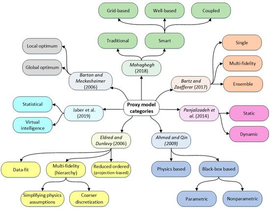
The most significant advantage of constructing a proxy model is the reduction in computational load and the time required for tasks such as uncertainty quantification, history matching, or production forecasting and optimization. According to the literature, different classes of proxy models exist, and there is no agreement on the proxy model categorization. Existing categories do not provide a comprehensive overview of all proxy model types with their applications in the oil and gas industry. Furthermore, a guideline to discuss the required steps to construct proxy models is needed. The proxy models in this work can fall into four groups: multi-fidelity, reduced-order, traditional proxy, and smart proxy models. The methodology for developing the multi-fidelity models is based on simplifying physics, and reduced-order models are based on the projection into a lower-dimensional. The procedure to develop traditional and smart proxy models is mostly similar, with some additional steps required for smart proxy models. Smart proxy models implement the feature engineering technique, which can help the model to find new hidden patterns within the parameters. As a result, smart proxy models generate more accurate results compared to traditional proxy models. Different steps for proxy modeling construction are comprehensively discussed in this review. For the first step, the objective of constructing a proxy model should be defined. Based on the objective, the related parameters are chosen, and sampling is performed. The sampling can be either stationary or sequential. Then, a new model is constructed between the considered inputs and outputs. This underlying model may be trained based on statistics, machine learning algorithms, simplifying physics, or dimensional reduction.