Your browser does not fully support modern features. Please upgrade for a smoother experience.
Please note this is a comparison between Version 2 by Beatrix Zheng and Version 1 by Yiming Shao.
Vertical farming is a new branch of urban agriculture using indoor vertical space and soil-less cultivation technology to obtain agricultural products. Despite its many advantages over traditional farming, it still faces some challenges and obstacles, including high energy consumption and costs, as well as uncertainty and a lack of social acceptance.
- vertical farming
- decomposed theory of planned behavior
- partial least squares structural equation modeling
- public acceptance
- behavioral intention
1. Introduction
The contemporary world, population expansion, and accelerating urbanization have become important reasons for the increase in the differences between agricultural land and construction land [1]. Apart from shrinking farmland, extreme weather caused by global climate change has had a huge impact on the traditional model of agricultural production, which has raised concerns about food security [2]. In 1999, Despommier introduced the concept of urban “vertical farming” and committed to promoting this new agricultural production mode to deal with the challenges of modern society [3].
The basic idea of vertical farming (VF) is to transform the original single-layer flat agricultural model into a multi-layer vertically stacked model that integrates modern agricultural technologies such as soil-less cultivation, artificial Light Emitting Diode (LED) sources, environmental control, and renewable energy to produce agriculture inside urban buildings [4]. Compared with traditional agriculture, the main advantages of VF include
-
Improving production efficiency while avoiding the impact of extreme weather on agricultural production and ensuring food safety due to the controlled indoor environment [6].
-
Reducing environmental pollution caused by agricultural production processes using renewable-energy-recycling technology and avoiding the use of pesticides [2].
-
Establishing urban “local food supply chains” as a supplement and buffer to long-distance food supply chains [7].
In addition, VF has certain ecological and environmental benefits. On the urban scale, large commercial VF is usually combined with resource reuse and recycling facilities, such as solid waste treatment, wastewater treatment, and waste heat recycling that enhance the sustainability of the city [9]. In terms of the indoor environment, the air purification effects of the main indoor air pollutants have been verified including carbon dioxide, particulate matter, and some volatile organic compounds [10]. VF also helps to improve the physical and psychological environment due to the visual relaxation effects of ecological designs [11]. In addition, it enhances indoor daylight distribution by providing shade and diffuse reflection in front of the windows [12].
Despite its potential advantages, the concept of VF has been met with skepticism and even criticism. First, due to cost-effective constraints, the types of plants suitable for vertical farming are limited. Leafy greens with high water content rather than crops high in carbohydrates are much more suitable plant species for VF since they grow much faster and consume fewer resources such as electricity and water [13,14][13][14]. Second, VF may bring about certain favorable or unfavorable effects on the indoor environment. For example, plant transpiration increases indoor relative humidity by 9–12% [10]. This may be favorable for indoor comfort in arid regions but could be disadvantageous in hot and humid regions [15]. Other considerations include the noise made by hydroponic systems [16], a minor chance of discomfort as a result of allergies [17], and energy consumption and heat dissipation caused by the artificial growth lights [18]. Finally, the exhaust gases, wastewater, and heat emitted from VF could affect the urban environment if not properly treated or recycled [16]. Currently, a series of solutions has been already tested and implemented to deal with the aforementioned challenges. For example, the cost-effectiveness of VF could be greatly enhanced by the careful selection of crop varieties and continuous improvements to the energy efficiency of the VF equipment and systems [19]. As for VF’s possible negative impacts on the environment, the integration of different systems and technologies is needed to reduce, reuse, or recycle the waste from VF [20].
Technology should not be an obstacle as it continues to improve. However, there are still uncertainties around the economic feasibility and social acceptance of VF. Shao et al. [21] developed the world’s first evaluation software to simulate VF’s economic feasibility and energy consumption considering the impact of multiple factors such as region, type, and technology level. The simulated results show that VF could be preferable in areas with high vegetable prices, low energy costs, and high labor costs, where the annual rate of return on investment can be up to 25%. Conversely, it could be easy to develop the project in a state of loss for a long time, thereby reducing commercial attractiveness. Zhang et al. [22] analyzed the economic feasibility of introducing VF to a university park. The results showed that the payback period of a 5000 m2 vertical farm was 11.5 years and that the annual profit could reach $92,000. Avgoustaki et al. [23] analyzed and compared the internal rate of return and the net present value of VF and greenhouses for the same planting area (225 m2). The restudyearch showed that VF was economically more advantageous. Its internal rate of return was 34.74% with a payback period of 4 years. In contrast, Graff [24] estimated the return on investment for a 10-storey vertical farm in Toronto to be only about 8%, which was below the minimum acceptable rate of 10–12% for most investors.
Compared with an economic feasibility analysis of agriculture-oriented VF, studies on the social acceptance of small-scale mixed-use VF, especially family-run or office-based micro-VF, are scarcely documented. Mixed-use VF can be used not only for agricultural purposes, but also for other functions such as recreation [25], education [26], decoration, and exhibitions [27]. For this type of VF, agricultural production is usually considered a value-added function rather than the main function. In mixed-use VF, occupants are often more concerned with the improvements to the quality of the indoor environment brought about by vertical farming than the annual yield of agricultural produce. Mixed-use VF with the most market potential are family farms since the proportion of residential land is usually the largest in cities. However, the uncertainty lies in public acceptance and the preference for consumption. In order to research and develop this market, this restudyearch applies surveys and information systems to provide an important basis for market forecast analysis, taking a comprehensive consideration of objective conditions and subjective willingness [28].
2. Theories and Models of Users’ Behavioral Intentions
In recent years, research on information systems applications has developed rapidly. The restudyearch of users’ behavioral intentions (BI) has become an important part of research on user acceptance [29]. Models and theories have been used to predict user behavior, including the Theory of Reasoned Action (TRA) [30], Theory of Planned Behavior (TPB) [31[31][32],32], and Decomposed Theory of Planned Behavior (DTPB) [33]. The TRA suggests that the execution of individual behavior is governed by BI [34], but this theory ignores the influence of objective reality on BI, resulting in its limited and questionable scope of application [34]. To compensate for the shortcomings of the TRA, Ajzen [35] incorporated Perceived Behavioral Control (PBC) into the theoretical model to form the TPB, which broadened the application area of the theory. However, as the research continued, many scholars found that the TPB has the same limitations as the TRA, and the belief dimensions of the two theories show multiple dimensions in many situations [36]. Accordingly, Taylor and Todd [37] combined the Diffusion of Innovation Theory (IDT) with the TPB in 1995 and proposed the DTPB using the second-order deconstruction of the three single linear structures in the TPB. Antecedent variables can be added or reduced in the model according to the specific research object and scenario, which is conducive to further explorations of the deeper psychological perceptual elements of individual behavior. Compared with the TRA and TPB, the DTPB has a broader perspective and greater explanatory power and applicability in multiple research fields, since a more stable belief structure can be built [38]. Therefore, although yet to be developed and applied in VF research, DTPB modeling could be an effective approach to investigating social acceptance and willingness to adopt VF.
3. Factors Influencing Acceptance and Willingness
From the perspective of behavioral theory, for individuals, acceptance and willingness to use new technologies are the result of the combined effects of various factors such as their socioeconomic attributes, social relationship norms, and behavioral control [39]. Studies have found that an individual’s attributes, such as gender, age, occupation, education level, income level, etc., have an impact on their willingness to use new technologies [40]. Studies have shown that people with higher income levels are more concerned about the quality of agricultural products than the price [41]. Younger groups are more receptive to and tolerant of new technologies. Women are more cautious in viewing and using new technologies than men [42]. As a new planting technology, the complexity of the planting process of vertical agriculture and the consumption of individual money, time, and energy in this process are also important factors that impact public planting intention. In addition, the advice and behavior of people around an individual are also important factors. Therefore, this paper first investigates the influence of an individual’s own socioeconomic attributes on planting intentions and then investigates the influence of other factors such as social relationship norms and behavior control.
There are two types of the disaggregate behavioral model of individual behavioral intentions [43]. RP (revealed preference) is an investigation of an individual’s completed choice behavior [44], and SP (stated preference) is an investigation of how an individual makes a choice and how he considers it under hypothetical conditions [45]. RP is for investigating the results and conditions of choices made by individuals in a certain actual state, mainly targeting actual or occurring schemes, that is, the contents of the survey are the observed behavioral choice data that have taken place [46]. SP is mainly used to investigate the factors and degree of influence that affect consumers’ acceptance of a product or service, and the main purpose is to obtain people’s subjective preferences for behavioral choices under assumed conditions that have not yet occurred [47]. Since there were no existing data on vertical agricultural planting behavior, the SP survey method was selected for this restudyearch.
4. Decomposed Theory of Planned Behavior
The DTPB is a type of SP survey method that uses behavior intention (BI) to measure public acceptance of and willingness to use new technologies. The DTPB suggests that BI can have a direct effect on an individual’s behavior. It means that a strong intention to perform a certain behavior indicates that an individual is more likely to perform that behavior [48]. Meanwhile, the DTPB assumes that BI is determined by three main constructs: behavioral attitude (BA), subjective norm (SN), and perceived behavioral control (PBC) [49]. These three components are expressed in behavioral decision contexts as behavioral beliefs, normative beliefs, and control beliefs. BA is an individual’s evaluation of a particular behavior [50]. SN specifically refers to the expectations that the individual perceives from the surrounding group, which may have a significant influence on the individual when making a certain behavioral decision [51]. PBC is a person’s perception of the ease or difficulty of performing a particular behavior. It is mainly expressed in the perceived ability of the individual to control the required resources and opportunities [52]. The relationship between BI and the three determinants, BA, SN, and PBC, has been supported by previous research [53]. In the context of the present restudyearch, positive feelings toward the use of VF can encourage the public to accept it. Being introduced to the concept by family, relatives, friends, or colleagues, or encouraged by elders or superiors, can influence the public’s behavior toward using VF. Similarly, skills and conditions that facilitate VF can influence the intention to adopt VF.
Behavioral belief refers to the possible results of VF perceived by the public, which is the determinant of BA [54]. Davis used PU and PEU in the TAM, which theorizes that an individual’s perception of system usefulness and ease of use influence his or her attitude toward system usage as well as his or her behavioral intention, which in turn determines system acceptance and its usage [55]. He defined PU as “the degree to which a person believes that using a particular system would enhance his or her job performance” and PEU as “the degree to which a person believes that using a particular system would be free from effort” [55]. In the planting process of vertical agriculture, PU can be redefined as the extent to which people perceive that VF can help them increase their income and improve their indoor environment, and even the extent to which VF plays a role in sustainable urban development; PEU represents the ease of mastering the planting process and operating the VF structure, as well as the convenience of accessing and navigating the intelligent control system. As for the indoor physical environment, VF will also have some negative effects. As well as the benefits, growers should also weigh the adverse effects of VF on their living or working environments.
Based on this, this preseaperrch deconstructs the behavioral beliefs into three constructs, PU, PEU, and PR, and selects four indicators to measure planting intention: economic benefits, environmental benefits, operational difficulties, and risk assessment. The higher the benefit of the planting behavior or the easier the grower perceives the planting operation to be, the stronger the attitude of the grower to perform the planting behavior; at the same time, the lower the negative impact of the planting behavior, the more positive the attitude of the grower to perform the planting behavior.
Normative beliefs refer to the public’s perceptions of the expectations of significant others or teams about whether they should participate in planting using VF, which is the determinant of SN [35]. In reality, when the public is unfamiliar with the various outcomes of planting using VF, they rely on the groups around them to form the basis for their own decisions by integrating the voices of all parties, which in turn facilitates the formation of SNs about the public’s willingness to accept and plant using VF. In this restudyearch, SN does not focus on social influences on decision making. SI comes from elders at home or leaders at work, whereas PI comes from family, friends, and colleagues [56].
Based on the above analysis, this preseaperrch deconstructs normative beliefs into two constructs, PI and SI, and selects five indicators, family, friends, colleagues, elders, and leaders, to measure planting willingness. The more positive encouragement from the surrounding groups, the greater the willingness of the public to engage in planting using VF.
Control belief refers to the factors that the public can perceive during the process of planting VF, which may promote or hinder this behavior [57]. This perception of control consists of two aspects: the internal aspect comes from the public’s perceptions of their own abilities, such as money and time, and the external aspect comes from the influence of the surrounding external forces on the public’s own behavior. In the process of planting, this external force mainly refers to convenience, that is, the sufficient degree of the resources that the public possesses in order to realize planting behavior, such as the VF product sales platform and planting knowledge learning platform, etc.
According to this analysis, this restudyearch deconstructs control beliefs into two constructs, SE and FC, corresponding to six indicators of planting knowledge, reserve, risk-aversion ability, time cost–tolerance, financial cost–tolerance, planting information acquisition ability, and product-trading-platform construction. The greater the public’s recognition of their own abilities or the more favorable the external facilitation conditions, the stronger their willingness to plant.
5. Partial Least Squares Structural Equation Modeling (PLS-SEM)
In recent years, as an important tool for multivariate data analysis, structural equation modeling (SEM) has become a mainstream method in the field of social science research [58]. Based on different research techniques, SEM can be divided into covariance-based structural equation modeling (CB-SEM) [59] and partial least squares structural equation modeling (PLS-SEM) [60]. Recently, PLS-SEM applications have expanded into marketing research and practice with the recognition that PLS-SEM’s distinctive methodological features make it a possible alternative to the more popular CB-SEM approaches [61]. Compared with CB-SEM, PLS-SEM has the following main advantages: (1) it requires fewer samples; (2) it can handle complex models with multiple latent variables; (3) it can handle both reflective and formative indicators; (4) it can handle non-constant information; and (5) it can reduce the impact of multicollinearity on modeling accuracy and reliability [62].
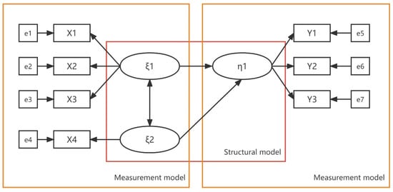
As shown in Figure 1, PLS-SEM consists of two parts. The first part is the measurement model, also known as the external model. The external model assesses the contribution of each indicator in representing its related underlying variables and evaluates the degree to which a set of indicators fits a potential variable. The second part is the structural model, also known as the internal model, which measures the direct and indirect relationships between latent variables [63]. Among them, X1… X4 and Y1… Y3 represent the observed variables, ξ1 and ξ2 are the latent exogenous variables, η1 represents the latent variables, and e1… e7 represent the error terms associated with the observed variables [64]. Among them, the relationships between ξ, X, and e and η, Y, and e can be expressed by Equations (1) and (2), respectively:
ξ=λ⋅X+e
η=λ⋅Y+e
where λ represents the path coefficient. In SEM, the relationship between the observed variable and the latent variable is a linear function; the meaning of the latent variable is reflected in the observed variable, and a change in the latent variable will lead to a change in the observed scalar.
As shown in Figure 2, the basic evaluation process of PLS-SEM is divided into two stages. The first stage evaluates the measurement model and the second stage evaluates the structural model. The measurement model assessment is mainly to test the quality of the theoretical models. Prior to beginning, researchers usually check the indicator loading of each variable. The minimum threshold value for the loadings is 0.70, which indicates that the construct explains over 50% of the indicators’ variances. The structural model assessment covers structural theory, including determining whether structural relationships are important and meaningful and then testing the hypotheses. Consistent with other analytical methods, PLS-SEM relies on empirical rules to evaluate the results estimated by the model. What follows is a discussion and description of the thresholds for each indicator.
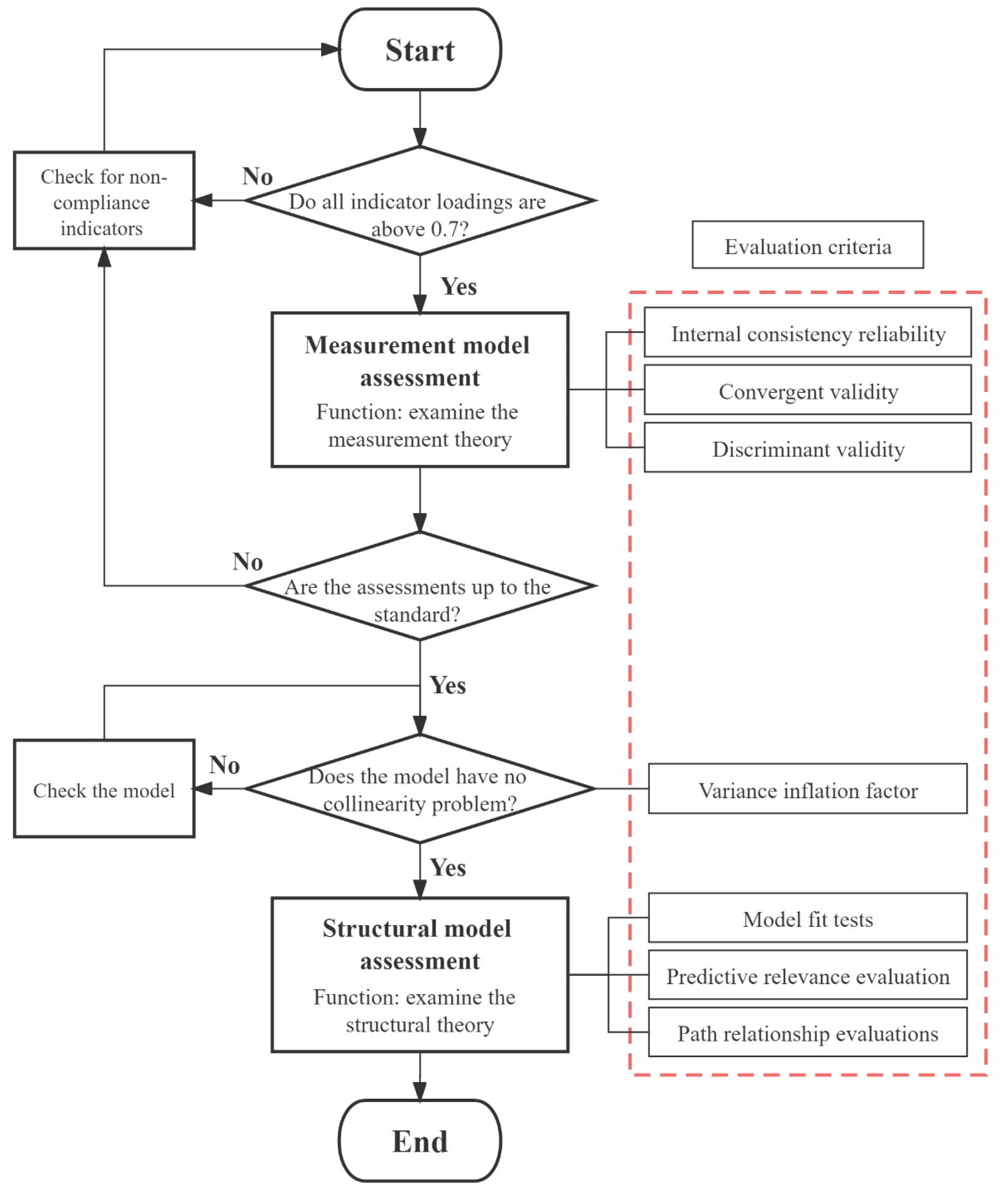
Figure 2. Workflow of PLS-SEM evaluation.
5.1. Measurement Model Assessment
The first step in the measurement model evaluation involves the assessment of the constructs’ internal consistency reliability. When using PLS-SEM, internal consistency reliability is typically evaluated using composite reliability (CR) and Cronbach’s alpha (CA) [65]. The values of CA and CR of all variables exceeding 0.7 assured reliability in the internal consistency among these constructs. However, CR values higher than 0.95 are considered problematic as they indicate that the items are redundant, leading to issues such as inflated correlations among the indicator error terms [66].
In the second step, the convergent validity of the measured constructs is examined. Convergent validity measures the extent to which a construct converges in its indicators by explaining the items’ variances [67]. Convergent validity is assessed by the average variance extracted (AVE) for all items associated with each construct. In the case of indicator loading and CR higher than 0.7, the recommended value of AVE is 0.50 or higher [68] as it indicates that on average, the construct explains over 50% of the variances in its items.
Once the reliability and convergent validities of the reflective constructs are successfully established, the final step is to assess the discriminant validities of the constructs. Discriminant validity refers to the extent to which a measure is distinct from other measures from which it is supposed to differ [58]. The most conservative criterion recommended to evaluate discriminant validity is the Fornell and Larcker criterion [69]. The method compares each construct’s AVE value with the squared inter-construct correlation of that construct with all other constructs in the structural model [70]. The evaluation criterion is that a construct should not exhibit shared variance with any other construct that is greater than its AVE value [71]. Another approach to assessing discriminant validity is to examine the cross-loadings [71]. The evaluation criterion for this approach is that an indicator variable should exhibit a higher loading on its own construct than on any other construct included in the structural model [71]. If the loadings of the indicators are consistently highest on the construct with which they are associated, then the construct exhibits discriminant validity.
5.2. Structural Model Assessment
The next step after having established the constructs’ validities is to examine the causal relationship among the latent constructs. This covers structural theory, which includes determining whether the structural relationships are significant and meaningful and then testing the hypotheses [71]. Prior to this assessment, researchers must test for potential collinearity between the structural model’s predictors. When the values of all variance inflation factors (VIF) are lower than 3.3, it indicates that there is no collinearity problem in the model [72].
The first step of the structural model evaluation is to test the goodness of fit of the model. This restudyearch adopted several criteria to assess the PLS-SEM model’s fit, including the standardized root mean square residual (SRMR), the squared Euclidean distance (d-ULS) and the geodesic distance (d-G), and the Normed Fit Index (NFI) [73]. The highest threshold of SRMR is 0.08 [74], whereas the recommended value of NFI is 0.7 and above [75].
Next, one of the important parts of evaluating an SEM is testing the predictive accuracy and predictive relevance of the model [76]. The predictive accuracy is tested using the coefficient of determination (R2 value), which presents the degree of variance explained in each endogenous construct. As explained by Hair et al. [77], a value of R2 ranging between 0 and 1 with a higher value of R2 indicated a higher level of predictive accuracy. Specifically, 0.19, 0.33, and 0.67, respectively, represent the three levels, small, medium, and large prediction accuracies [78]. Another means of assessing a model’s predictive relevance is the Q2, also known as blindfolding [79]. This method is based on the blindfolding procedure of PLS-SEM 3.0. As a rule of thumb, Q2 values greater than zero for a particular endogenous construct indicate that the model’s predictive accuracy is acceptable for that particular construct [71].
Finally, the strength and significance of the path coefficients are evaluated for the relationships hypothesized between the constructs. Generally, the direct and indirect relationships among the constructs are evaluated using regression coefficients (β) [59]. In terms of relevance, β values are standardized on a range from −1 to +1, with coefficients closer to +1 representing strong positive relationships and coefficients closer to −1 indicating strong negative relationships [71]. In addition, the bootstrap procedure was conducted to assess the significance of the β values in the indirect relationships among the constructs based on the t-value and p-value. When the t-value is higher than 1.96 or the p-value is less than 0.05, the path relationship is considered to be significant at the 95% significance level [80,81][80][81].
References
- Besthorn, F.H. Vertical Farming: Social Work and Sustainable Urban Agriculture in an Age of Global Food Crises. Aust. Soc. Work. 2013, 66, 187–203.
- La Rosa, D.; Barbarossa, L.; Privitera, R.; Martinico, F. Agriculture and the city: A method for sustainable planning of new forms of agriculture in urban contexts. Land Use Policy 2014, 41, 290–303.
- Despommier, D. The Rise of Vertical Farms. Sci. Am. 2009, 301, 80–87.
- Marris, E. The Vertical Farm: Feeding the World in the 21st Century. Nature 2010, 468, 374.
- Malochleb, M. Vertical farming to gain ground. Food Technol. Chic. 2019, 73, 10–11.
- Despommier, D. The vertical farm: Controlled environment agriculture carried out in tall buildings would create greater food safety and security for large urban populations. J. Fur Verbrauch. Lebensm. 2011, 6, 233–236.
- Al-Kodmany, K. The Vertical Farm: A Review of Developments and Implications for the Vertical City. Buildings 2018, 8, 24.
- Al-Chalabi, M. Vertical farming: Skyscraper sustainability? Sustain. Cities Soc. 2015, 18, 74–77.
- Vaughan, A. Is vertical farming the way to a greener life? New Sci. 2019, 242, 15.
- Shao, Y.; Li, J.; Zhou, Z.; Hu, Z.; Zhang, F.; Cui, Y.; Chen, H. The effects of vertical farming on indoor carbon dioxide concentration and fresh air energy consumption in office buildings. Build. Environ. 2021, 195, 107766.
- Langemeyer, J.; Madrid-Lopez, C.; Mendoza Beltran, A.; Villalba Mendez, G. Urban agriculture—A necessary pathway towards urban resilience and global sustainability? Landsc. Urban Plan. 2021, 210, 104055.
- Wong, C.E.; Zhi, W.; Shen, L.; Yu, H. Seeing the lights for leafy greens in indoor vertical farming. Trends Food Sci. Tech. 2020, 106, 48–63.
- Santini, A.; Bartolini, E.; Schneider, M.; Vinicius, G.D.L. The crop growth planning problem in vertical farming. Eur. J. Oper. Res. 2021, 294, 377–390.
- Li, Y.; Wang, C.; Zhu, S.; Yang, J.; Wei, S.; Zhang, X.; Shi, X. A Comparison of Various Bottom-Up Urban Energy Simulation Methods Using a Case Study in Hangzhou, China. Energies 2020, 13, 4781.
- Shao, Y.; Li, J.; Zhou, Z.; Zhang, F.; Cui, Y. The Impact of Indoor Living Wall System on Air Quality: A Comparative Monitoring Test in Building Corridors. Sustainability 2021, 13, 7884.
- Safikhani, T.; Abdullah, A.M.; Ossen, D.R.; Baharvand, M. A review of energy characteristic of vertical greenery systems. Renew. Sustain. Energy Rev. 2014, 40, 450–462.
- Kalantari, F.; Tahir, O.M.; Joni, R.A.; Fatemi, E. Opportunities and Challenges in Sustainability of Vertical Farming: A Review. J. Landsc. Ecol. 2018, 11, 35–60.
- Yusof, S.; Thamrin, N.M.; Nordin, M.K.; Yusoff, A.; Sidik, N.J. Effect of artificial lighting on typhonium flagelliforme for indoor vertical farming. In Proceedings of the 2016 IEEE International Conference on Automatic Control and Intelligent Systems (I2CACIS), Shah Alam, Malaysia, 22 October 2016.
- Touliatos, D.; Dodd, I.C.; McAinsh, M. Vertical farming increases lettuce yield per unit area compared to conventional horizontal hydroponics. Food Energy Secur. 2016, 5, 184–191.
- Tan Gar Heng, A.; Bin Mohamed, H.; Bin Mohamed Rafaai, Z.F. Implementation of lean manufacturing principles in a vertical farming system to reduce dependency on human labour. Int. J. Adv. Trends Comput. Sci. Eng. 2020, 9, 512–520.
- Shao, Y.; Heath, T.; Zhu, Y. Developing an economic estimation system for vertical farms. Int. J. Agric. Environ. Inf. Syst. 2016, 7, 26–51.
- Zhang, H.; Asutosh, A.; Hu, W. Implementing Vertical Farming at University Scale to Promote Sustainable Communities: A Feasibility Analysis. Sustainability 2018, 10, 4429.
- Avgoustaki, D.D.; Xydis, G. Indoor Vertical Farming in the Urban Nexus Context: Business Growth and Resource Savings. Sustainability 2020, 12, 1965.
- Graff, G. Skyfarming. In Bachelor Type; University of Waterloo: Waterloo, ON, Canada, 2011.
- Pascual, M.P.; Lorenzo, G.A.; Gabriel, A.G. Vertical Farming Using Hydroponic System: Toward a Sustainable Onion Production in Nueva Ecija, Philippines. Open J. Ecol. 2018, 8, 25–41.
- Khalil, H.I.; Wahhab, K.A. Advantage of vertical farming over horizontal farming in achieving sustainable city, Baghdad city-commercial street case study. IOP Conf. Ser. Mater. Sci. Eng. 2020, 745, 12115–12173.
- Mo, Z.; Bonenberg, W.; Xia, W.; Liu, S. How Vertical Farming Influences Urban. Landscape Architecture and Sustainable Urban. Developments. In Proceedings of the International Conference on Applied Human Factors and Ergonomics, Orlando, FL, USA, 22–26 July 2018.
- Baliga, S.; Vohra, R. Market Research and Market Design. Adv. Theor. Econ. 2010, 3, 1059.
- Compeau, D.R.; Higgins, C.A.; Huff, S.L. Social cognitive theory and individual reactions to computing technology. MIS Q. 1999, 23, 145–158.
- Ajzen, I. Theory of reasoned action. Cloth. Text. Res. J. 2000, 25, 244–257.
- Botetzagias, I.; Dima, A.F.; Malesios, C. Extending the theory of planned behavior in the context of recycling: The role of moral norms and of demographic predictors. Resour. Conserv. Recycl. 2015, 95, 58–67.
- Papaoikonomou, K.; Latinopoulos, D.; Emmanouil, C.; Kungolos, A. A Survey on Factors Influencing Recycling Behavior for Waste of Electrical and Electronic Equipment in the Municipality of Volos, Greece. Environ. Processes 2020, 7, 321–339.
- Shih, Y.; Fang, K. The use of a decomposed theory of planned behavior to study Internet banking in Taiwan. Internet Res. 2004, 14, 213–223.
- Hill, R. Belief, Attitude, Intention and Behavior: An Introduction to Theory and Research.by Martin Fishbein; Icek Ajzen. Contemp. Sociol. 1977, 6, 244–245.
- Ajzen, I. The theory of planned behavior. Organ. Behav. Hum. Dec. 1991, 50, 179–211.
- Davis, V.F.D. A Theoretical Extension of the Technology Acceptance Model: Four Longitudinal Field Studies. Manag. Sci. 2000, 46, 186–204.
- Taylor, S.; Todd, P.A. Understanding Information Technology Usage: A Test of Competing Models. Inf. Syst. Res. 1995, 6, 144–176.
- Chang, I.C.; Chou, P.C.; Yeh, K.J.; Tseng, H.T. Factors influencing Chinese tourists’ intentions to use the Taiwan Medical Travel App. Telemat. Inform. 2016, 33, 401–409.
- Poston, D.L.; Jing, S. Women entrepreneurship in relation to psychological demographic and socioeconomic Attributes. Popul. Dev. Rev. 2012, 13, 703.
- Eleonora, P.; Di, P.L. Understanding Consumer’s Acceptance of Technology-Based Innovations in Retailing. J. Technol. Manag. Innov. 2012, 7, 1–19.
- Annunziata, A.; Scarpato, D. Factors affecting consumer attitudes towards food products with sustainable attributes. Agric. Econ. 2014, 60, 353–363.
- Tacken, M.; Marcellini, F.; Mollenkopf, H.; Ruoppila, I.; Széman, Z. Use and acceptance of new technology by older people: Findings of the international MOBILATE survey ‘Enhancing mobility in later life’. Gerontechnology 2005, 3, 126–137.
- Hirobata, Y.; Kawakami, S. Modeling disaggregate behavioral modal switching models based on intention data. Transp. Res. Part. B Methodol. 1990, 24, 15–25.
- Stavins, R.N. The Costs of Carbon Sequestration: A Revealed-Preference Approach. Am. Econ. Rev. 1999, 89, 994–1009.
- Bateman, I.; Carson, R.; Day, B.; Hanemann, W.; Hanley, N.; Hett, T.; Joneslee, M.; Loomes, G.; Mourato, S.; Ozdemiroolu, E. Economic Valuation with Stated Preference Techniques. Ecol. Econ. 2004, 50, 155–156.
- Varian, H.R. Revealed preference with a subset of goods. J. Econ. Theory 1988, 46, 179–185.
- Adamowicz, W.; Boxall, P.; Williams, M.; Louviere, J. Stated Preference Approaches for Measuring Passive Use Values: Choice Experiments and Contingent Valuation. Am. J. Agric. Econ. 1998, 80, 64–75.
- Ajzensupa Supsup Sup, I. The theory of planned behaviour: Reactions and reflections. Psychol. Health 2011, 26, 1113–1127.
- Shiue, Y.-M. Investigating the Sources of Teachers′ Instructional Technology Use through the Decomposed Theory of Planned Behavior. J. Educ. Comput. Res. 2007, 36, 425–453.
- Manstead, A.S.R. Attitudes and Behaviour. Appl. Soc. Psychol. 1996, 20, 3–29.
- Wetzels, S.M. A meta-analysis of the technology acceptance model: Investigating subjective norm and moderation effects. Inf. Manag. Amster 2007, 44, 90–103.
- Gellman, M.D.; Turner, J.R. Perceived Behavioral Control; Springer: New York, NY, USA, 2013.
- Yousafzai, S.Y.; Foxall, G.R.; Pallister, J.G. Technology acceptance: A meta-analysis of the TAM: Part 1. J. Model. Manag. 2007, 2, 251–280.
- Taylor, S.; Todd, P. Decomposition and crossover effects in the theory of planned behavior: A study of consumer adoption intentions. Int. J. Res. Mark. 1995, 12, 137–155.
- Davis, F.D. Perceived Usefulness, Perceived Ease of Use, and User Acceptance of Information Technology. MIS Q. 1989, 13, 319–340.
- Smarkola, C. A Mixed-Methodological Technology Adoption Study; Teo T. Technology Acceptance in Education; Sense Publishers: Rotterdam, The Netherlands, 2011; pp. 9–41.
- Ajzen, I. From Intentions to Actions: A Theory of Planned Behavior; Springer: Berlin/Heidelberg, Germany, 1985.
- Hair, J.F. Multivariate Data Analysis: An Overview; Springer: Berlin/Heidelberg, Germany, 2011.
- Hair, J.F.; Gabriel, M.; Patel, V. AMOS Covariance-Based Structural Equation Modeling (CB-SEM): Guidelines on its Application as a Marketing Research Tool. Soc. Sci. Electron. Publ. 2015, 13, 44–55.
- Sarstedt, M.; Ringle, C.M.; Hair, J.F. Partial Least Squares Structural Equation Modeling; Springer International Publishing: New York, NY, USA, 2014.
- Ringle, C.M.; Sarstedt, M.; Straub, D. A Critical Look at the Use of PLS-SEM in MIS Quarterly. Soc. Sci. Electron. Publ. 2012, 36, iii–xiv.
- Hair, J.F.; Sarstedt, M.; Ringle, C.M.; Mena, J.A. An assessment of the use of partial least squares structural equation modeling in marketing research. J. Acad. Mark. Sci. 2012, 40, 414–433.
- Hair, J.; Hollingsworth, C.L.; Randolph, A.B.; Chong, A. An updated and expanded assessment of PLS-SEM in information systems research. Ind. Manag. Data Syst. 2017, 117, 442–458.
- Sarstedt, M.; Ringle, C.M.; Smith, D.; Reams, R.; Hair, J.F. Partial least squares structural equation modeling (PLS-SEM): A useful tool for family business researchers. J. Fam. Bus. Strateg. 2014, 5, 105–115.
- Mann, S. Research Methods for Business: A Skill-Building Approach. Leadersh. Org. Dev. J. 2013, 34, 700–701.
- Drolet, A.L.; Morrison, D.G. Do We Really Need Multiple-Item Measures in Service Research? J. Serv. Res. Us. 2001, 3, 196–204.
- Straub, D.; Gefen, D. Validation Guidelines for IS Positivist Research. Commun. Assoc. Inf. Syst. 2004, 13, 24.
- Hair, J.F.; Black, W.C.; Babin, B.J.; Anderson, R.E. Multivariate Data Analysis: A Global Perspective; Pearson Education: Essex, UK, 2010.
- Hamid, M.A.; Sami, W.; Sidek, M.M. Discriminant Validity Assessment: Use of Fornell & Larcker criterion versus HTMT Criterion. J. Phys. Conf. 2017, 890, 12163.
- Sarstedt, M.; Hair, J.F.; Ringle, C.M.; Thiele, K.O.; Gudergan, S.P. Estimation issues with PLS and CBSEM: Where the bias lies! J. Bus. Res. 2016, 69, 3998–4010.
- Ketchen, D.J. A Primer on Partial Least Squares Structural Equation Modeling. Long Range Plan. 2013, 46, 184–185.
- Akinwande, M.O.; Dikko, H.G.; Samson, A. Variance Inflation Factor: As a Condition for the Inclusion of Suppressor Variable(s) in Regression Analysis. Open J. Stat. 2015, 5, 754–767.
- Henseler, J.; Hubona, G.; Ray, P.A. Using PLS path modeling in new technology research: Updated guidelines. Ind. Manag. Data Syst. 1980, 116, 2–20.
- Henseler, J.; Ringle, C.M.; Sarstedt, M. Testing Measurement Invariance of Composites Using Partial Least Squares. Soc. Sci. Electron. Publ. 2015, 49, 41–46.
- Hu, L.T.; Be Ntler, P.M. Fit indices in covariance structure modeling: Sensitivity to underparameterized model misspecification. Psychol. Methods 1998, 3, 424–453.
- Hair, J.F.; Ringle, C.M.; Gudergan, S.P.; Fischer, A.; Nitzl, C.; Menictas, C. Partial least squares structural equation modeling-based discrete choice modeling: An illustration in modeling retailer choice. Bus. Res. 2019, 12, 115–142.
- Hair, J.; Astrachan, C.B.; Moisescu, O.I.; Radomir, L.; Ringle, C.M. Executing and Interpreting Applications of PLS-SEM: Updates for Family Business Researchers. J. Fam. Bus. Strateg. 2020, 12, 100392.
- Henseler, J.; Ringle, C.M.; Sinkovics, R.R. The Use of Partial Least Squares Path Modeling in International Marketing; Emerald Group Publishing Ltd.: Bingley, UK, 2009; Volume 20, pp. 227–319.
- Rigdon, E.E. Rethinking Partial Least Squares Path Modeling: Breaking Chains and Forging Ahead. Long Range Plann. 2014, 47, 161–167.
- Driessen, T.; Tijs, S.H. The t-value, the core and semiconvex games. Int. J. Game Theory 1985, 14, 229–247.
- Rice, W.R. A Consensus Combined P-Value Test and the Family-Wide Significance of Component Tests. Biometrics 1990, 46, 303–308.
More