This contribution assesses a new term that is proposed to be established within Land Change Science: Spatio-TEmporal Patterns of Land (‘STEPLand’). It refers to a specific workflow for analyzing land-use/land cover (LUC) patterns, identifying and modeling driving forces of LUC changes, assessing socio-environmental consequences, and contributing to defining future scenarios of land transformations. Researchers define this framework based on a comprehensive metaanalysis of 250 selected articles published in international scientific journals from 2000 to 2019. The empirical results demonstrate that STEPLand is a consolidated protocol applied globally, and the large diversity of journals, disciplines, and countries involved shows that it is becoming ubiquitous. The main characteristics of STEPLand are provided and discussed, demonstrating that the operational procedure can facilitate the interaction among researchers from different fields, and communication between researchers and policy makers.
- LUCC patterns
- spatial modeling of driving forces
- socio-environmental consequences
- future scenarios
- In-deep reading analysis
1. Introduction
2. STEPLand Framework
STEPLand is defined as an operation framework typical of LCS, and composed of four steps, moving from broader to narrower epistemological perspectives (Figure 1):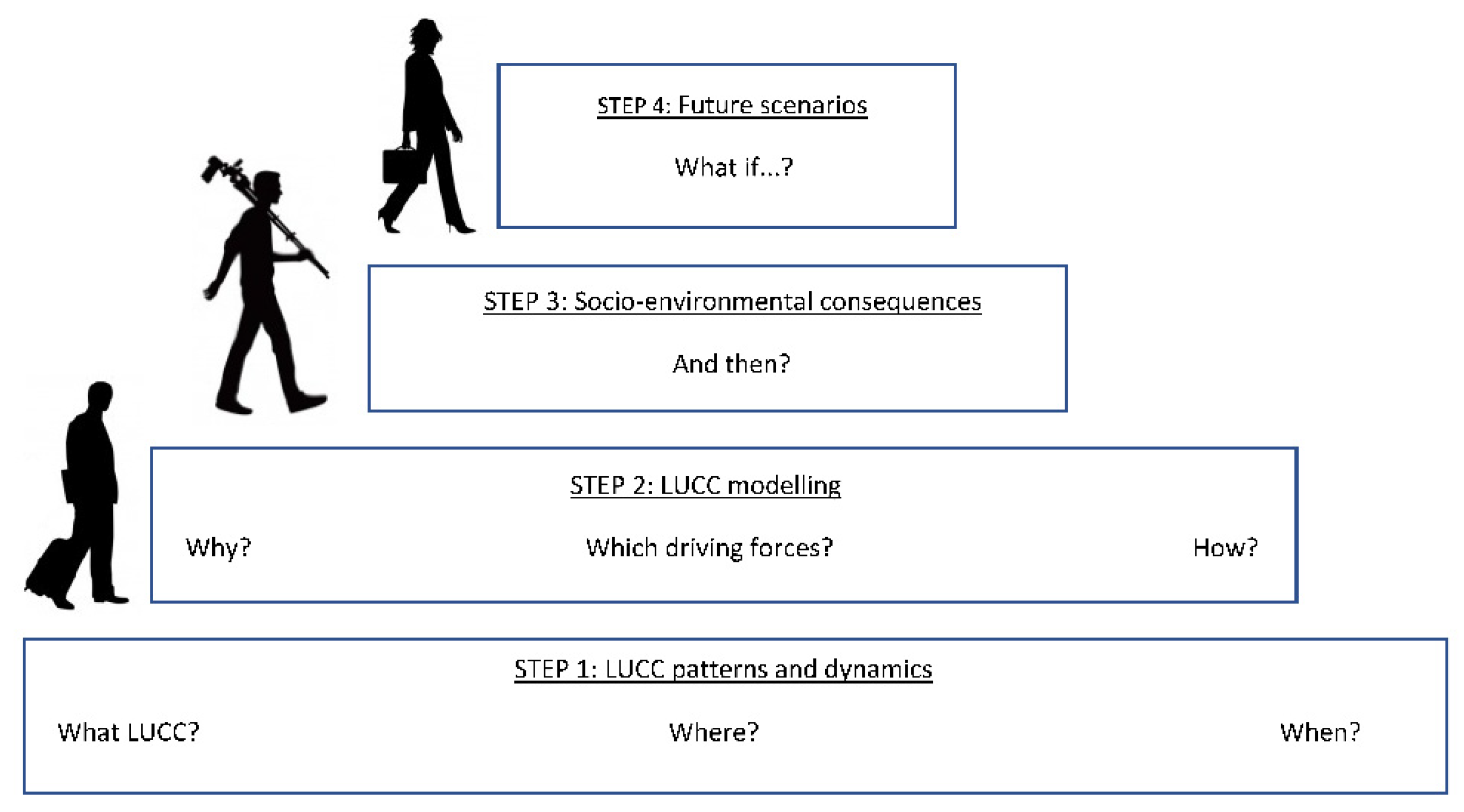
2.1. LUCC Patterns and Dynamics
The first step of STEPLand includes a formal assessment and characterization of LUCC, mainly based on Earth Observation (EO) techniques, e.g., remote sensing (RS). EO and GIS data facilitate trans-sectoral research and provide a platform for integrating multiple information layers that may include ancillary (or validation) data [14][15]. RS tools provide valuable multitemporal data for monitoring LUCC patterns and processes at different spatial scales (local, regional, national, continental, and global), and GIS techniques make it possible to analyze them explicitly [16][17][18]. Spatial, spectral, and radiometric RS resolutions affect the size, condition, and precision of the explicit features to be discriminated in a landscape scene, whereas the temporal resolution of satellite imagery determines the intrinsic territorial, environmental, and socio-economic dynamics of local systems [10][19][20][21]. Both dimensions represent large technical challenges. During the past 40 years, significant advances in sensor technologies have improved the spatial, spectral, radiometric, and temporal resolutions, and the coverage, of satellite imagery [22]. The classification phase is the process of identifying spectral similarities in the multidimensional spectral space and linking them to LUC categories. This involves assigning pixels to different LUC classes identified in a given study. Diverse classification taxonomy options are now available but, traditionally, these have been divided according to the pixel technique used (per-pixel or sub-pixel), or according to the application of training samples (supervised methods or unsupervised methods), among others [23][24][25]. Similarity in spectral reflectance properties of natural surfaces at a given moment often impedes consistent identification and mapping of a large range of LUC, such as agricultural crops or individual communities constituted by natural vegetation. Furthermore, the spectral response of many cover types varies throughout the year: LUC categories that appear similar in spring may become distinguishable at earlier or later stages of the annual cycle. Therefore, a multi-temporal approach based on large RS databases is more suitable for revealing the complex LUC patterns characteristic, for instance, of the Mediterranean Basin [26][27][28]. In order to minimize the classification errors due to seasonal changes, an appropriate strategy is to select images from the same month or, at least, from the same season [29][30]. After a classification is obtained, the next step is to assess the accuracy or how well a classification has worked. This assessment measures the correlation between satellite imagery classification and ground reference samples to quantify the overall agreement between RS classification (global accuracy and user and producer accuracy by categories) and ground truthing data [31]. Once LUC maps are generated and tested, among the available change detection techniques, the most usual method is the post-classification or map-to-map comparison (i.e., a comparative analysis of independently produced LUC classifications from different dates) associated with a transition or change matrix [32][33]. According to [34], post-classification is an accurate procedure that bypasses the difficulties associated with analyzing images acquired at different times of the year or by different sensors, and thus delineating the nature of change [35]. Nevertheless, this method has two well-known critical issues [36][37]: first, misregistration of the polygon boundaries (locational inaccuracy) in the different classifications, and, therefore, the presence of border pixels with false positive or negative changes. With rasters, this is basically the consequence of non-matching pixels [38]; with vector shapes, this problem is known as “sliver”, i.e., narrow polygons of uncertain interpretation [39][40][41]. The second issue relates to problems derived from classification errors: a false positive change may be recorded when no change has taken place because a pixel in one map (or in both maps) is misclassified, or false negative changes, when no change is identified but a change has taken place in the field. Therefore, this approach requires a good accuracy level in both classification maps because the change map accuracy is the product of the accuracies of the individual classifications, and therefore, it is subject to error propagation [42][43][44].2.2. LUCC Modeling
Modeling is a process that provides a platform for encoding inferred (or deduced) relationships, thus allowing simulations and projections based on mathematical (algorithmic) specifications or procedures [45]. LUCC modeling is a tool for supporting planners and policymakers in developing robust policies and decisions. At the same time, models can be used to provide an ex ante assessment of policies or serve as an early warning system for environmental impacts. Six conceptual dimensions are considered to be particularly important for carrying out LUCC modeling [46]: (i) analysis level, (ii) cross-scale dynamics, (iii) driving forces, (iv) spatial interactions and neighborhood effects, (v) temporal dynamics, and (vi) level of data integration. In general terms, LUCC is often modeled as a function of a selection of socio-economic and biophysical variables acting as driving forces that shape land change [2][47][48][49]. Modeling LUCC driving forces comprises a wide variety of methodological approaches, which can be classified in different ways. For instance, [3] divided driving forces into three groups: socio-economic drivers, biophysical drivers, and land management variables; [50] differentiated proximate causes, those actions that directly affect land use, such as wood extraction, from underlying causes, i.e., those “fundamental forces” that underpin the proximate causes, including demographic, economic, technological, institutional, and cultural factors [51]. In general, Ref. [52] identified five driving forces: (i) biophysical constraints and potentials, (ii) economic factors, (iii) social factors, (iv) spatial policies, and (v) spatial interactions and neighborhood characteristics. Others [48][53][54] differentiated actors of change from driving forces. Actors are the decision-making and mediating agents, including individuals (e.g., farmers), households, neighborhoods, agencies (e.g., planning organizations), and institutions, whereas driving forces are the (sometimes materialized) expression of their decisions or acts, e.g., through laws, subsidies, or incentives [55]. Moreover, Ref. [53] provided a specific definition of the “spatial domain” as the institutional (and geographical) context where a given agent interacts with the landscape (e.g., countries, regions, prefectures/provinces, municipalities). Representation of the domain can be facilitated in a geographically explicit model using boundary maps or vector layers. The extent of the study area also influences the selection: larger areas imply a diversification of LUC contexts and may require analyzing a larger variety of driving forces. Therefore, the analysis scale (local, regional, national, or global) can produce a specific representation based on different driving forces. For instance, the presence of small ecologically valuable areas can be the main determinant of LUCC patterns at a local scale, whereas the distance from the market can be a more important factor at a regional scale [46]. Specification and quantification of the intrinsic relationship between driving forces and LUCC are particularly important in model implementation. According to [56], modelers should select the drivers or explanatory variables that are supposed to play an active role in land change. Even in automated approaches, input variables are selected based on expert knowledge, although data availability (e.g., the lack of data for some economic variables, such as land ownership, or, for earlier times, e.g., gross domestic product in 1850) is often a major limitation, as documented in [57]. According to [45], models used for LUCC analysis range from those oriented towards pattern description/recognition to those quantifying and interpreting dynamics. One study [58] provided a more generalized classification, arguing that models can be static or dynamic, spatial or non-spatial, inductive or deductive, and/or agent-based or pattern-based (e.g., emulation of individual decision makers vs. inference of the underlying behavior derived from LUCC patterns). Models can use a large range of information (satellite imagery, official statistics, maps or field surveys, among others) often implemented in GIS and eventually combined in composite indicators. Actor-based, bottom-up models based on household surveys represent the land change agent explicitly by emulating individual decision makers through agent-based approaches. Land evaluation pattern-based top-down models use RS and census data to simulate LUCC through parameterized transition equations that convert land from one cover type to another [59]. Finally, Ref. [60] separated inductive pattern-based models from cellular automata approaches, sector-based economic models, spatially disaggregated economic approaches, and agent-based models. Therefore, driving forces form a tangled system of interactions that affect multiple temporal and spatial levels, making it difficult to carry out adequate analyses and obtain representation systems. Combining data from the social and natural sciences is a particularly complicated task due to the different operational scales, the complexity in relating social science data to a specific geographic place, and the difficulty involved in integrating qualitative data, which is more common in social science, and less common in ecological disciplines [47]. Moreover, driving forces—and not only LUCC—are also subject to changes, which influence the identification of representative study periods, and thus affects the model’s results [61]. Precision of statistical methodologies and data availability are also important. As a summary, identification of LUCC drivers (sensu [26]) implies (i) the clarification of latent relationships between landscape patterns and driving forces (explorative models), and (ii) the projection of future landscapes under different scenarios (predictive models). Two of the main issues arising when socio-economic and biophysical variables are combined spatially, as a process of data integration or data equalization [62][63][64] characteristic of STEPLand, are the different data formats and spatial scales. Socio-economic data are usually available from official statistics in tabular format at some administrative boundaries: neighborhoods, districts, census tracks, municipalities, regions, and countries, among others [65][66]. By comparison, biophysical variables are mainly extracted from EO sources, from spatial interpolation techniques (e.g., exploiting point data derived from climate stations) or from other sources (e.g., rasterization of archive maps) having a specific pixel size [67]. When the two types of data are combined, these issues may lead to a loss in spatial precision [68], given the need to integrate data at one specific scale, namely, according to administrative boundaries (i.e., native vector file) or to lattices (i.e., raster file with a given pixel size). As socio-economic data are mostly available for administrative areas, an option is to convert biophysical data into class intervals and calculate the area (or percentage) occupied by each interval within the appropriate spatial (polygon) domain. For instance, Ref. [69] adopted the area option, whereas [70] calculated the proportion of three different intervals of slopes within each district, and adopted a similar solution for soil moisture. Another study [71] clipped LUC data to the boundaries of each of the 25 watersheds considered in the study, and then calculated zonal statistics for each watershed to extract the relative proportions of each LUC type for subsequent use in statistical analyses. Another option is to calculate the mean value of cardinal variables per spatial (polygon) domain, thus producing a high generalization. It is also possible to assign central (median) or dominant (mode) values for each administrative area. This latter option is appropriate for discrete variables, such as soil type. When the option is to work at a pixel size, the problem is the inverse, as it affects the socio-economic data: a rasterization is required in order to match the pixel size of biophysical variables and LUCC. The main issue in this case is whether a statistical analysis is applied because all the pixels included in the administrative boundary have the same socio-economic value, showing a maximum spatial autocorrelation, which leads to a violation of the assumption of independent residuals. To minimize this situation, a convenient “solution” is to apply a “reduced factor” through, for instance, a stratified random sampling at a lower number of pixels. This option was applied in [72] using a “contraction factor” amounting to 10. Another option is “data generalization”, e.g., using a grid lattice having larger pixel sizes, which is representative of a lower spatial resolution; for example, in [73], all the variables describing deforestation and the respective drivers of change were aggregated to 25 km grid cells.2.3. Socio-Environmental Consequences
The third step of STEPLand takes the socio-environmental consequences of LUCC into account. For instance, LUCC may affect weather and climate variability by altering biophysical, biogeochemical, and energy exchange processes at local, regional, and global scales. Therefore, the consequences of these processes are scale-dependent because some of them affect the local environment (e.g., local water quality), whereas other impacts extend far beyond the location where they arise (e.g., carbon cycle, climate change). Because not all LUCCs have global effects, and LUCCs are not irreversible, there are several multi-directional impacts that can reinforce, mitigate, or offset multiple consequences, enriching the debate regarding on-site and off-site factors of change [74][75]. One specific repercussion considered in this review is related to landscape, given its particular nature because it contributes significantly to well-being and quality of life. Quantification of spatio-temporal landscape dynamics and the underlying drivers is key for planning appropriate decisions in this field [76]. Landscape metrics are common tools for measuring spatial changes in landscape composition and configuration, including fragmentation and diversity [77]. From a STEPLand perspective, they can be applied to RS and GIS data and simultaneously used with LUCC models and statistical methods. There are several quantitative measures, for example, those in [78], that can be used to assess landscape composition, such as the number of patches (patch richness) and uniformity and variety (evenness and diversity), and to assess the configuration or the spatial distribution of patches in the landscape (landscape pattern); these include patch shape, isolation, spread between classes (contagion), mean patch size, and density. Another additional consequence considered in STEPLand is the impact on ecosystem services because, in recent years, these services have attracted the increasing attention of researchers, policymakers, and other stakeholders worldwide [79]. The main reason for this is that, when land is used, society changes and modifies the quantity and quality of the provision of these services. According to [80], supply and demand of ecosystem services can be assessed at, and transferred to, different spatial and temporal scales by linking LUCC (e.g., extracted from remote sensing) with other data (e.g., obtained from interviews). Their results reveal patterns of human activities over time and space, and the capacities of different ecosystems to provide ecosystem services under changing LUC. However, Ref. [81] reviewed the “ecosystem services” concept and the various methods applied for mapping and assessing quantitative methods, and the significant problem of there not being a clear distinction between services, functions, and benefits.2.4. Futures Scenarios
The last stage included in the STEPLand perspective corresponds to the simulation and prediction of future LUCC scenarios. This is a significant process for policy makers because it enables them to better anticipate actions, especially in the context of urban planning and the protection of natural land [82]. A previous study [83] provided a literature review of models applied to predict LUCC, including Markov chains (MCs), landscape models, CLUE-S models, cellular automata (CA), integration of Markov chains and cellular automata (MC-CA), and artificial neural networks. Markov chains, for instance, quantify LUCC probabilities between different states that are recorded in a transition matrix [84]. This matrix is the result of cross-tabulation between satellite images derived from two sequential dates, adjusted by proportional error and translated into a set of probability images, one for each LUC category [85][86]. In addition, CA models are one of the most relevant tools for understanding complex systems, particularly LUC patterns, given their intrinsic sensitivity to both spatial configuration and neighborhood relationships. The future state of the cells is determined by the current state of the cell itself and that of the neighborhood cells, following transition functions based on a set of rules. A variety of methods has been used for calculating transition rules in CA, such as logistic regression, multinomial logit, linear and geometric formulations, support vector machines, and, more recently, artificial neural networks [87].References
- Turner, B.L., II; Lambin, E.F.; Reenberg, A. The emergence of land change science for global environmental change and sustainability. Proc. Natl. Acad. Sci. USA 2007, 104, 20666–20671.
- Brissoulis, H. Analysis of Land Use Change: Theoretical and Modeling Approaches, 2nd ed.; Loveridge, S., Jackson, R., Eds.; Regional Research Institute, West Virginia University: Morgantown, WV, USA, 2020; Available online: https://researchrepository.wvu.edu/rri-web-book/3 (accessed on 8 May 2020).
- Turner, B.L., II; Skole, D.; Sanderson, S.; Fischer, G.; Fresco, L.; Leemans, R. Land-Use and Land-Cover Change: Science/Research Plan; IGBP Report 35; IGBP/HDP; Royal Swedish Academy of Sciences: Stockholm, Sweden; Geneva, Switzerland, 1995.
- Seitzinger, S.P.; Gaffney, O.; Brasseur, G.; Broadgate, W.; Ciais, P.; Claussen, M.; Erisman, J.W.; Kiefer, T.; Lancelot, C.; Monks, P.S.; et al. International Geosphere–Biosphere Programme and Earth system science: Three decades of co-evolution. Anthropocene 2015, 12, 3–16.
- Arino, O.; Bicheron, P.; Achard, F.; Latham, J.; Witt, R.; Weber, J.L. Globcover: The Most Detailed Portrait of Earth; European Space Agency Bulletin: Frascati, Italy, 2008; Volume 136.
- Justice, C.; Gutman, G.; Vadrevu, K.P. NASA Land Cover and Land Use Change (LCLUC): An interdisciplinary research program. J. Environ. Manag. 2015, 148, 4–9.
- Verburg, P.H.; Crossman, N.; Ellis, E.C.; Heinimann, A.; Hostert, P.; Mertz, O.; Nagendra, H.; Sikor, T.; Erb, K.-H.; Golubiewski, N.; et al. Land system science and sustainable development of the earth system: A global land project perspective. Anthropocene 2015, 12, 29–41.
- Rounsevell, M.D.A.; Pedroli, B.; Erb, K.-H.; Gramberger, M.; Busck, A.G.; Haberl, H.; Kristensen, S.; Kuemmerle, T.; Lavorel, S.; Lindner, M.; et al. Challenges for land system science. Land Use Policy 2012, 29, 899–910.
- Gutman, G.; Janetos, A.C.; Justice, C.O.; Moran, E.F.; Mustard, J.F.; Rindfuss, R.R.; Skole, D.; Turner, B.L., II; Cochrane, M.A. Land Change Science: Observing, Monitoring and Understanding Trajectories of Change on the Earth’s Surface; Kluwer Academic Publishers: Dordrecht, The Netherlands, 2004.
- Rindfuss, R.R.; Walsh, S.J.; Turner, B.L., II; Fox, J.; Mishra, V. Developing a science of land change: Challenges and methodological issues. Proc. Natl. Acad. Sci. USA 2004, 101, 13976–13981.
- Bajocco, S.; Dragoz, E.; Gitas, I.; Smiraglia, D.; Salvati, L.; Ricotta, C. Mapping forest fuels through vegetation phenology: The role of coarse-resolution satellite time-series. PLoS ONE 2015, 10, e0119811.
- Rindfuss, R.R.; Entwisle, B.; Walsh, S.J.; An, L.; Badenoch, N.; Brown, D.G.; Deadman, P.; Evans, T.P.; Fox, J.; Geoghegan, J.; et al. Land use change: Complexity and comparisons. J. Land Use Sci. 2008, 3, 1–10.
- Meyfroidt, P.; Chowdhury, R.R.; de Bremond, A.; Ellis, E.C.; Erb, K.-H.; Filatova, T.; Garrett, R.D.; Grove, J.M.; Heinimann, A.; Kuemmerle, T.; et al. Middle-range theories of land system change. Glob. Environ. Change 2018, 53, 52–67.
- Baynard, C.W. Remote sensing applications: Beyond land-use and land-cover change. Adv. Remote Sens. 2013, 2, 228–241.
- Nagabhatla, N.; Padmanabhan, M.; Kühle, P.; Vishnudas, S.; Betz, L.; Niemeyer, B. LCLUC as an entry point for transdisciplinary research–Reflections from an agriculture land use change study in South Asia. J. Environ. Manag. 2015, 148, 42–52.
- Long, H.; Tang, G.; Li, X.; Heilig, G.K. Socio-economic driving forces of land-use change in Kunshan, the Yangtze River Delta economic area of China. J. Environ. Manag. 2007, 83, 351–364.
- Uddin, K.; Chaudhary, S.; Chettri, N.; Kotru, R.; Murthy, M.; Chaudhary, R.P.; Ning, W.; Shrestha, S.M.; Gautam, S.K. The changing land cover and fragmenting forest on the Roof of the World: A case study in Nepal’s Kailash Sacred Landscape. Landsc. Urban Plan. 2015, 141, 1–10.
- Gómez, C.; White, J.C.; Wulder, M.A. Optical remotely sensed time series data for land cover classification: A review. ISPRS J. Photogramm. Remote Sens. 2016, 116, 55–72.
- Serra, P.; Pons, X. Monitoring farmers’ decisions on Mediterranean irrigated crops using satellite image time series. Int. J. Remote Sens. 2008, 29, 2293–2316.
- Wulder, M.A.; Masek, J.G.; Cohen, W.B.; Loveland, T.R.; Woodcock, C.E. Opening the archive: How free data has enabled the science and monitoring promise of Landsat. Remote Sens. Environ. 2012, 122, 2–10.
- Kuemmerle, T.; Erb, K.; Meyfroidt, P.; Muller, D.; Verburg, P.H.; Estel, S.; Haberl, H.; Hostert, P.; Jepsen, M.R.; Kastner, T.; et al. Challenges and opportunities in mapping land use intensity globally. Curr. Opin. Environ. Sustain. 2013, 5, 484–493.
- Sishodia, R.; Ray, R.L.; Singh, S.K. Applications of Remote Sensing in Precision Agriculture: A Review. Remote Sens. 2020, 12, 3136.
- Lu, D.; Weng, Q. A survey of image classification methods and techniques for improving classification performance. Int. J. Remote Sens. 2007, 28, 823–870.
- Gilani, H.; Shrestha, H.L.; Murthy, M.S.R.; Phuntso, P.; Pradhan, S.; Bajracharya, B.; Shrestha, B. Decadal land cover change dynamics in Bhutan. J. Environ. Manag. 2015, 148, 91–100.
- Phiri, D.; Morgenroth, J. Developments in Landsat land cover classification methods: A review. Remote Sens. 2017, 9, 967.
- Alvarez-Martinez, J.M.; Suárez-Seoanea, S.; De Luis Calabuig, E. Modelling the risk of land cover change from environmental and socio-economic drivers in heterogeneous and changing landscapes: The role of uncertainty. Landsc. Urban Plan. 2011, 101, 108–119.
- Serra, P.; Pons, X. Two Mediterranean irrigation communities in front of water scarcity: A comparison using satellite image time series. J. Arid Environ. 2013, 98, 41–51.
- Kibret, K.S.; Marohn, C.; Cadisch, G. Assessment of land use and land cover change in South Central Ethiopia during four decades based on integrated analysis of multi-temporal images and geospatial vector data. Remote Sens. Appl. Soc. Environ. 2016, 3, 1–19.
- Clement, F.; Orange, D.; Williams, M.; Mulley, C.; Epprecht, M. Drivers of afforestation in Northern Vietnam: Assessing local variations using geographically weighted regression. Appl. Geogr. 2009, 29, 561–576.
- Ariti, A.T.; van Vliet, J.; Verburg, P.H. Land-use and land-cover changes in the Central Rift Valley of Ethiopia: Assessment of perception and adaptation of stakeholders. Appl. Geogr. 2015, 65, 28–37.
- Foody, G.M. Status of land cover classification accuracy assessment. Remote Sens. Environ. 2002, 80, 185–201.
- Pontius, R.G.; Shusas, E.; McEachern, M. Detecting important categorical land changes while accounting for persistence. Agric. Ecosyst. Environ. 2004, 101, 251–268.
- Cuba, N. Research note: Sankey diagrams for visualizing land cover dynamics. Landsc. Urban Plan. 2015, 139, 163–167.
- Mas, J.F. Monitoring land-cover changes: A comparison of change detection techniques. Int. J. Remote Sens. 1999, 20, 139–152.
- Dewan, A.M.; Yamaguchi, Y.; Rahman, M.Z. Dynamics of land use/cover changes and the analysis of landscape fragmentation in Dhaka Metropolitan, Bangladesh. GeoJournal 2012, 77, 315–330.
- Aspinall, R.J.; Hill, M.J. Land cover change: A method for assessing the reliability of land cover changes measured from remotely-sensed data. In Proceedings of the International Geoscience and Remote Sensing Symposium, IGARSS ’97, Singapore, 4–8 August 1997; pp. 269–271.
- Serra, P.; Pons, X.; Saurí, D. Post-classification change detection with data from different sensors. Some accuracy considerations. Int. J. Remote Sens. 2003, 24, 3311–3340.
- Szabó, S.; Bertalan, L.; Kerekes, A.; Novák, T.J. Possibilities of land use change analysis in a mountainous rural area: A methodological approach. Int. J. Geogr. Inform. Sci. 2016, 30, 708–726.
- Chrisman, N.R. The accuracy of map overlays: A reassessment. Landsc. Urban Plan. 1987, 14, 427–439.
- Goodchild, M.F.; Guoqing, S.; Shiren, Y. Development and test of an error model for categorical data. Int. J. Geogr. Inf. Systems 1992, 6, 87–104.
- Frondoni, R.; Mollo, B.; Capotorti, G. A landscape analysis of land cover change in the Municipality of Rome (Italy): Spatio-temporal characteristics and ecological implications of land cover transitions from 1954 to 2001. Landsc. Urban Plan. 2011, 100, 117–128.
- Singh, A. Digital change detection techniques using remotely-sensed data. Int. J. Remote Sens. 1989, 10, 989–1003.
- Lambin, E.F.; Strahler, A.H. Change vector analysis in multitemporal space: A tool to detect and categorize land-cover change processes using high temporal resolution satellite data. Remote Sens. Environ. 1994, 48, 231–244.
- Were, K.O.; Dick, Ø.B.; Singh, B.R. Remotely sensing the spatial and temporal land cover changes in Eastern Mau forest reserve and Lake Nakuru drainage basin, Kenya. Appl. Geogr. 2013, 41, 75–86.
- Brown, D.G.; Verburg, P.H.; Pontius, R.G., Jr.; Lange, M. Opportunities to improve impact, integration, and evaluation of land change models. Curr. Opin. Environ. Sustain. 2013, 5, 452–457.
- Verburg, P.; Ritsema van Eck, J.; de Nijs, T.; Dijst, M.; Schot, P. Determinants of land use change patterns in the Netherlands. Environ. Plan. B Urban Anal. City Sci. 2004, 31, 125–150.
- Bürgi, M.; Hersperger, A.M.; Schneeberger, N. Driving forces of landscape change–Current and new directions. Landsc. Ecol. 2004, 19, 857–868.
- Hersperger, A.M.; Gennaio, M.P.; Verburg, P.H.; Bürgi, M. Linking land change with driving forces and actors: Four conceptual models. Ecol. Soc. 2010, 15, 1. Available online: http://www.ecologyandsociety.org/vol15/iss4/art1/ (accessed on 25 February 2020).
- Dang, A.N.; Kawasaki, A. A review of methodological integration in land-use change models. Int. J. Agric. Environ. Inf. Syst. 2016, 7, 1–25.
- Geist, H.J.; Lambin, E.F. What Drives Tropical Deforestation? A Meta-Analysis of Proximate and Underlying Causes of Deforestation Based on Subnational Case Study Evidence; Land-Use and Land-Cover Change (LUCC). Project IV. International Human Dimensions Programme on Global Environmental Change (IHDP); International Geosphere-Biosphere Programme (IGBP); LUCC International Project Office: Louvain-la-Neuve, Belgium, 2001.
- Serneels, S.; Lambin, E.F. Proximate causes of land-use change in Narok District, Kenya: A spatial statistical model. Agric. Ecosyst. Environ. 2001, 85, 65–81.
- Verburg, P.H.; Schot, P.P.; Dijst, M.J.; Veldkamp, A. Land use change modelling: Current practice and research priorities. GeoJournal 2004, 61, 309–324.
- Agarwal, C.; Green, G.L.; Grove, M.; Evans, T.; Schweik, C. A Review and Assessment of Land-Use Change Models: Dynamics of Space, Time and Human Choice; General Technical Report NE-297; United States Department of Agriculture, Indiana University: Bloomington, IN, USA, 2000.
- Schneeberger, N.; Bürgi, M.; Hersperger, A.M.; Ewald, K.C. Driving forces and rates of landscape change as a promising combination for landscape change research—An application on the northern fringe of the Swiss Alps. Land Use Policy 2007, 24, 349–361.
- Valbuena, D.; Verburg, P.H.; Bregt, A.K.; Ligtenberg, A. An agent-based approach to model land-use change at a regional scale. Landsc. Ecol. 2010, 25, 185–199.
- Mas, J.F.; Paegelow, M.; Camacho Olmedo, M.T. LUCC modeling approaches to calibration. In Geomatic Approaches for Modeling Land Change Scenarios; Camacho Olmedo, M.T., Paegelow, M., Mas, J.-F., Escobar, F., Eds.; Springer International Publishing: Cham, Switzerland, 2018; pp. 11–25.
- Parcerisas, L.L.; Marull, J.; Pino, J.; Tello, E.; Coll, F.; Basnou, C. Land use changes, landscape ecology and their socioeconomic driving forces in the Spanish Mediterranean coast (El Maresme County, 1850–2005). Environ. Sci. Policy 2012, 23, 120–132.
- Mas, J.F.; Kolb, M.; Paegelow, M.; Camacho Olmedo, M.T.; Houet, T. Inductive pattern-based land use/cover change models: A comparison of four software packages. Environ. Model. Softw. 2014, 51, 94–111.
- Pérez-Vega, A.; Mas, J.F.; Ligmann-Zielinska, A. Comparing two approaches to land use/cover change modeling and their implications for the assessment of biodiversity loss in a deciduous tropical forest. Environ. Model. Softw. 2012, 29, 11–23.
- Camacho Olmedo, M.T.; Paegelow, M.; Mas, J.-F.; Escobar, F. Geomatic Approaches for Modeling Land Change Scenarios; Springer International Publishing: Cham, Switzerland, 2018.
- Kolb, M.; Mas, J.F.; Galicia, L. Evaluating drivers of land-use change and transition potential models in a complex landscape in Southern Mexico. Int. J. Geogr. Inform. Sci. 2013, 27, 1804–1827.
- Entwisle, B.; Walsh, S.J.; Rindfuss, R.R.; Chamratrithirong, A. Land-use/land-cover and population dynamics, Nang Rong, Thailand. In People and Pixels. Linking Remote Sensing and Social Science; Liverman, D., Moran, E.F., Rindfuss, R.R., Stern, P.C., Eds.; National Academy Press: Washington, DC, USA, 1998; pp. 121–144.
- Walsh, S.J.; Crews-Meyer, K.A. Linking People, Place and Policy: A GIScience Approach; Kluwer Academic Publishers: Norwell, MA, USA, 2002.
- Fox, J.; Rindfuss, R.R.; Walsh, S.J.; Mishra, V. People and the Environment; Kluwer Academic Publishers: Boston, MA, USA, 2004.
- Zambon, I.; Colantoni, A.; Carlucci, M.; Morrow, N.; Sateriano, A.; Salvati, L. Land quality, sustainable development and environmental degradation in agricultural districts: A computational approach based on entropy indexes. Environ. Impact Assess. Rev. 2017, 64, 37–46.
- Salvati, L.; Ciommi, M.T.; Serra, P.; Chelli, F.M. Exploring the spatial structure of housing prices under economic expansion and stagnation: The role of socio-demographic factors in metropolitan Rome, Italy. Land Use Policy 2019, 81, 143–152.
- Bajocco, S.; Ceccarelli, T.; Smiraglia, D.; Salvati, L.; Ricotta, C. Modeling the ecological niche of long-term land use changes: The role of biophysical factors. Ecol. Indic. 2016, 60, 231–236.
- Wood, C.H.; Skole, D. Linking satellite, census, and survey data to study deforestation in the Brazilian Amazon. In People and Pixels. Linking Remote Sensing and Social Science; Liverman, D., Moran, E.F., Rindfuss, R.R., Stern, P.C., Eds.; National Academy Press: Washington, DC, USA, 1998; pp. 70–93.
- Perz, S.G.; Skole, D.L. Social determinants of secondary forests in the Brazilian Amazon. Soc. Sci. Res. 2003, 32, 25–60.
- Reger, B.; Otte, A.; Waldhardt, R. Identifying patterns of land-cover change and their physical attributes in a marginal European landscape. Landsc. Urban Plan. 2007, 81, 104–113.
- Shupe, S. Statistical and Spatial Analysis of Land Cover Impact on Selected Metro Vancouver, British Columbia Watersheds. Environ. Manag. 2013, 51, 18–31.
- Monteiro, A.T.; Fava, F.; Hiltbrunner, E.; Marianna, G.D.; Bocchi, S. Assessment of land cover changes and spatial drivers behind loss of permanent meadows in the lowlands of Italian Alps. Landsc. Urban Plan. 2011, 100, 287–294.
- Espindola, G.M.; de Aguiar, A.P.D.; Pebesma, E.; Câmara, G.; Fonseca, L. Agricultural land use dynamics in the Brazilian Amazon based on remote sensing and census data. Appl. Geogr. 2012, 32, 240–252.
- Chhabra, A.; Geist, H.; Houghton, R.A.; Haberl, H.; Braimoh, A.K.; Vlek, P.L.G.; Patz, J.; Xu, J.; Ramankutty, N.; Coomes, O.; et al. Multiple impacts pof land-use/cover change. In Land-Use and Land-Cover Change. Local Processes and Global Impacts; Lambin, E.F., Geist, H., Eds.; Springer: Heidelberg, Germany, 2006; pp. 71–116.
- Salvati, L.; Gemmiti, R.; Perini, L. Land degradation in Mediterranean urban areas: An unexplored link with planning? Area 2012, 44, 317–325.
- Dadashpoor, H.; Azizi, P.; Moghadas, M. Land use change, urbanization, and change in landscape pattern in a metropolitan area. Sci. Total Environ. 2019, 655, 707–719.
- Wu, Y.; Li, S.; Yu, S. Monitoring urban expansion and its effects on land use and land cover changes in Guangzhou city, China. Environ. Monit. Assess. 2016, 188, 54.
- McGarigal, K.; Cushman, S.; Ene, E. FRAGSTATS v4: Spatial Pattern Analysis Program for Categorical and Continuous Maps. 2012. Available online: https://www.umass.edu/landeco/research/fragstats/fragstats.html (accessed on 25 May 2021).
- Arowolo, A.O.; Deng, X.; Olatunji, O.A.; Obayelu, A.E. Assessing changes in the value of ecosystem services in response to land-use/land-cover dynamics in Nigeria. Sci. Total Environ. 2018, 636, 597–609.
- Burkhard, B.; Kroll, F.; Nedkov, S.; Müller, F. Mapping ecosystem service supply, demand and budgets. Ecol. Indic. 2012, 21, 17–29.
- Kertész, A.; Nagy, L.A.; Balázs, B. Effect of land use change on ecosystem services in Lake Balaton Catchment. Land Use Policy 2019, 80, 430–438.
- Basse, R.M.; Omrani, H.; Charif, O.; Gerber, P.; Bódis, K. Land use changes modelling using advanced methods: Cellular automata and artificial neural networks. The spatial and explicit representation of land cover dynamics at the cross-border region scale. Appl. Geogr. 2014, 53, 160–171.
- Aburas, M.M.; Ahamad, M.S.S.; Omar, N.Q. Spatio-temporal simulation and prediction of land-use change using conventional and machine learning models: A review. Environ. Monit. Assess. 2019, 205, 191–205.
- Hu, Y.; Batunacun; Zhen, L.; Zhuang, D. Assessment of land-use and land-cover change in Guangxi, China. Sci. Rep. 2019, 9, 2189.
- Garcia-Frapolli, E.; Ayala-Orozco, B.; Bonilla-Moheno, M.; Espadas-Manrique, C.; Ramos-Fernández, G. Biodiversity conservation, traditional agriculture and ecotourism: Land cover/land use change projections for a natural protected area in the northeastern Yucatan Peninsula, Mexico. Landsc. Urban Plan. 2007, 83, 137–153.
- Marshall, E.; Randhir, T.O. Spatial modeling of land cover change and watershed response using Markovian cellular automata and simulation. Water Resour. Res. 2008, 44, 1–10.
- Omrani, H.; Charif, O.; Gerber, P.; Bódis, K.; Basse, R.M. Simulation of Land Use Changes Using Cellular Automata and Artificial Neural Network; Working Paper No. 2012-01; CEPS/INSTEAD: Luxembourg, 2012.