Clustering is an attribute of a stationary stochastic process with an arbitrary marginal distribution function and a power-type dependence structure in large temporal and/or spatial scales yielding a high probability of low- (or high-) magnitude events to gather together in time and/or space. This behaviour of a stochastic process resembles that of a great variety of natural processes.
If spatial clustering is examined within a stationary framework, there may be an evolution of clustering in time which can be investigated and visualized by plotting of spatial climacograms in different timeframes.
- stochastic method
- clustering
- evolution of clustering
1. History
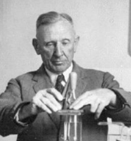
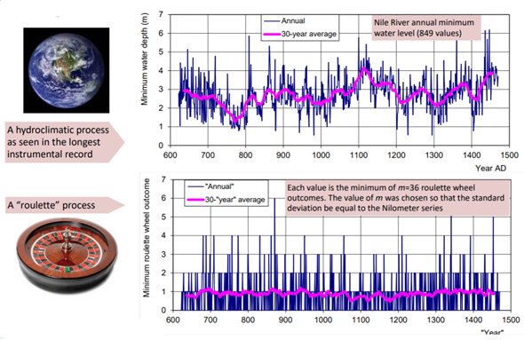
Clustering in nature has been first identified by H.E. Hurst (1951) [1] (Figure 1a) while studying the long-term behaviour in a variety of scales of the discharge timeseries of the Nile River in the framework of developing engineering projects in its basin.
Particularly, H.E. Hurst discovered a tendency of high-discharge years to cluster into high-flow periods, and low-discharge years to cluster into low-flow periods. This behaviour, also known as the Hurst phenomenon or Joseph effect (Mandelbrot, 1977) [2], has been verified in a variety of hydrological [3], hydrometeorological and turbulent processes [4] [5] and in other geophysical and alternate fields such as finance, medicine [6], and art [7] [8] [9].
All these processes are characterized by long-term persistence (LTP), which leads to high unpredictability in long-term scales due to the clustering of events as compared to the purely random process, i.e. white-noise (e.g. as in a fair dice game [10]), or other short-range dependence models (e.g., Markov).
 |
 |
| (a) | (b) |
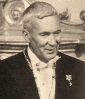
Figure 1: (a) In 1951 H.E. Hurst discovered the clustering behaviour in nature (b) A.N.Kolmogorov proposed a decade before a stochastic process that describes this clustering behaviour.
The mathematical description of the Hurst phenomenon is attributed to A.N. Kolmogorov (Figure 1b) who developed it while studying turbulence in 1940 [11] (Figure 1b), inspiring D. Koutsoyiannis [12] to name the general behaviour of the Hurst phenomenon as Hurst-Kolmogorov (HK) dynamics (Figure 2), to give credit to both contributing scientists and to distinguish it from the Gaussian LTP processes (e.g., fractional-Gaussian-noise [13]), and to incorporate alternate short-range dependence (e.g., Markov-behaviour [14]).
Figure 2. Hurst-Kolmogorov (HK) dynamics and the perpetual change of Earth’s climate
The HK dynamics has been recently also linked to the entropy maximization principle, and thus, to robust physical justification [15]. The stochastic simulation of the HK dynamics has been a mathematical challenge since it requires the explicit preservation of high-order moments in a vast range of scales, affecting both the intermittent behaviour in small scales [16] and the dependence in extremes [17] as well as the trends often appearing in geophysical timeseries [18].
2. Introduction
2.1 General
The mathematical field of Stochastics has been introduced on the opposite side of deterministic approaches, as a way to model the so-called random, i.e., complex, unexplained or unpredictable, fluctuations observed in non-linear geophysical processes. Such processes are marked by high unpredictability which gives rise to clustering structures appearing at various spatio-temporal scales. The existence of clustering can be claimed to be ubiquitous in the physical world, as it is found in galaxies, in ecosystems, in the societies of humans and animals, and even in the mere biological organization of life. Seen from a stochastic viewpoint, the anthropogenic world is also marked by the emergence of various types of clustering in space, increasing and decreasing in time, ranging from the mere organization of life in societies (e.g., urbanization) to the development of large-scale infrastructure and policies.
In the literature, there are many approaches to quantify clustering, calibrated for application in different fields as biology and ecosystems [19] [20], life sciences [21], [22], [23], [24], neural networks [25] physics and physical phenomena [26], [27], maps [28], [29] and more [30], yet there is no approach proposing a unifying stochastic view of 2D clustering in terms of variability vs. scale. Moreover, while the presence of 2D clustering is studied as a behavior, its temporal evolution is less explored as until recently, there was a scarcity of spatial information in time.
This stochastic methodology quantifies clustering in 2D space and its temporal evolution by analyzing image sequences of the spatial structures over time.[31]
2.2 Climacogram basics
Climacogram is a simple statistical tool to quantify change across time scales [32] [33]. It is. defined as the (plot of) variance of the averaged process (assuming stationary) versus averaging. The expression of the climacogram in one dimension is presented in figure 3, and in two dimensions is presented in figure 4, 5.
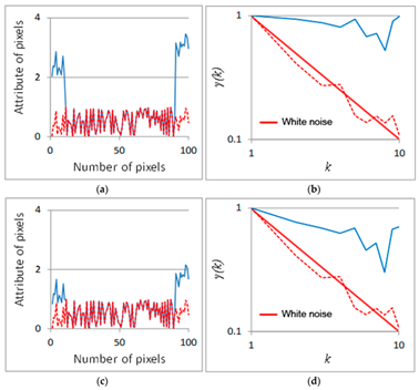
Figure 3. (a,c) Examples of data series with different statistical characteristics in one dimension; (b,d) Standardized climacograms of the data series shown in (a,c).
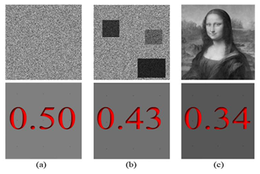
Figure 4. Examples of data series with different statistical characteristics in two dimensions;(a) White noise; (b) Simulated image with clustering behaviour; (c) Art painting. The lower row depicts the average brightness in the upper one.
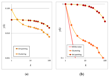
Figure 5. (a) Climacograms of the images described in Figure 3; (b) Standardized climacograms of the images in Figure 3.
3. Data model application and influences
3.1 Stochastic analysis of clustering in 2D space: the 2D-C tool
2D-C is a stochastic computational tool that measures the degree of variability (change in variability vs. scale) in images using stochastic analysis. Here, we refer to spatial scale, defined as the ratio of the area of k × k adjacent cells (i.e., scale k) that are averaged to form the (scaled) spatial field, over the spatial resolution of the original field (i.e., at scale 1).
Image processing typically begins with filtering or enhancing an image using techniques to extract more information from the images [34] and image segmentation is one of the basic problems in image analysis. The importance and utility of image segmentation have resulted in extensive research and numerous proposed approaches based on intensity, color, texture, etc., both automatic and interactive.
This analysis for image processing is based on a stochastic tool called the climacogram. The term climacogram [35] [36] comes from the Greek word climax (meaning scale). It is defined as the (plot of) variance of the averaged process (assuming stationary) versus averaging scale k and is denoted as γ(k). The climacogram is useful for detecting both the short- and the long-range change (or else dependence, persistence, clustering) of a process, with the latter emerging particularly in complex systems as opposed to white-noise (absence of dependence) or Markov (i.e., short-range dependence) behaviour [37].
In order to quantify the image variability, each image is first digitized in two dimensions (2D) based on grayscale color intensity (thus, studying the brightness of an image), and the climacogram is calculated based on the geometric scales of adjacent pixels. Assuming that our sample is an area nΔ × nΔ, where n is the number of intervals (e.g., pixels) along each spatial direction and Δ is the discretization unit (determined by the image resolution, e.g., pixel length), the empirical classical estimator of the climacogram for a 2D process can be expressed as:
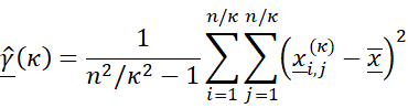
where the ‘^’ over γ denotes estimate, κ is the dimensionless spatial scale, xi,j(κ) represents the local average of the space-averaged process at scale κ and at grid cell (i, j), and, and uperlined x is the global average (underlined variables represent random variables as opposed to regular ones). Note that the maximum available scale for this estimator is n/2. The difference between the value in each element and the field average is raised to the power of 2, since we are mostly interested in the magnitude of the difference rather than its sign, and in particular, in the variance estimation. Therefore, the 2D-C expresses the diversity in color intensity among different elements at each scale by quantifying their variability of the brightness intensity.
An important property of stochastic processes that characterizes the variability over scales is the Hurst–Kolmogorov (HK) behavior (persistence), which can be represented by the Hurst parameter [38]. This parameter is estimated by minimizing the fitting error between the empirical (observed) and the modeled climacogram, both derived from the large-scale values, i.e., the last 50 scales are used in the presented applications of images). The isotropic HK process, i.e., the power-law decay of variance as a function of scale, with an arbitrary marginal distribution, is defined for a 1D or 2D process as:
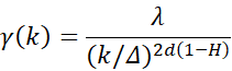
where γ is the variance at scale k, Δ is the time or space unit, d is the dimensionality of the process/field (i.e., for a 1D process d = 1, for a 2D field d = 2, etc.), and H is the Hurst parameter (0 < H < 1). For 0 < H < 0.5 the HK process exhibits an anti-persistent behavior, while H = 0.5 corresponds to the white noise process, and for 0.5 < H < 1 the process exhibits persistence (i.e., clustering), a common phenomenon in hydrometeorological processes (such as temperature, precipitation, wind etc), but also in other fiels such as landscapes [39] and art [7]. In this analysis, the clustering attribute is mostly due to the heterogeneity of the brightness of the examined images, where the high variability in brightness persists even in large scales. This clustering effect may substantially increase the diversity between the brightness in each pixel of the image.
An algorithm that can generate the climacogram in 2D was developed in MATLAB for rectangular images. In particular, for the current analysis, the images are cropped to 400 × 400 pixels, 14.11 cm × 14.11 cm, in 72 dpi (dots per inch).
3.2 Temporal evolution of 2D clustering
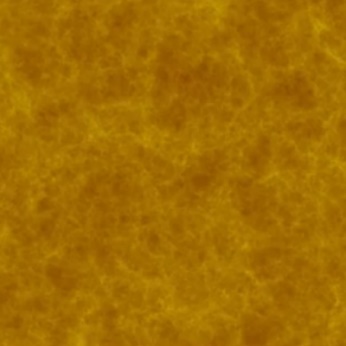
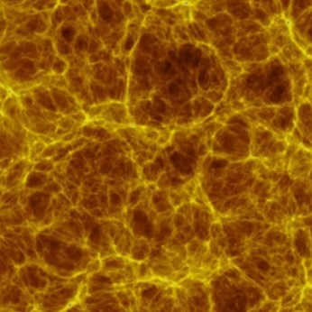
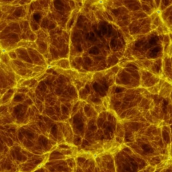
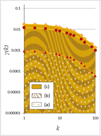
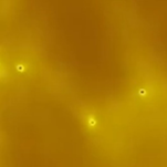
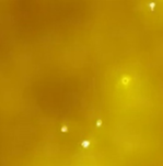
The pixels analyzed are represented by numbers denoting their color intensity in grayscale (white = 1, black = 0). Figure 6 presents images from three timeframes of the evolution of the universe as generated by a cosmological model of evolution [40]: (a) 500 million years after Big Bang, an image with faint clustering; (b) 1000 million years after Big Bang, an image with mild clustering, and (c) 10 000 million years after Big Bang, an image with intense clustering. Figure 7 depicts the scaled images at scales k = 2, 4, 8, 16, 20, 25, 40, 50, 80, 100 and 200, which are used to calculate the 2D-climacogram.
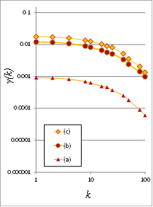
The presence of clustering is reflected in the climacogram (Figure 8a, 8b), which shows a marked difference as variance increases. Specifically, the variance of the images is notably higher at the scales with higher clustering, indicating a greater degree of variability of the process at these scales.
 |
 |
 |
| (a) | (b) | (c) |
Figure 6. Benchmark of image analysis, the evolution of the universe [40] [41]: (a) 500 million years after Big Bang image with faint clustering, average brightness 0.45; (b) 5000 million years after Big Bang image with clustering, average brightness 0.37 and (c) 10000 million years after Big Bang image with intense clustering, average brightness 0.33.
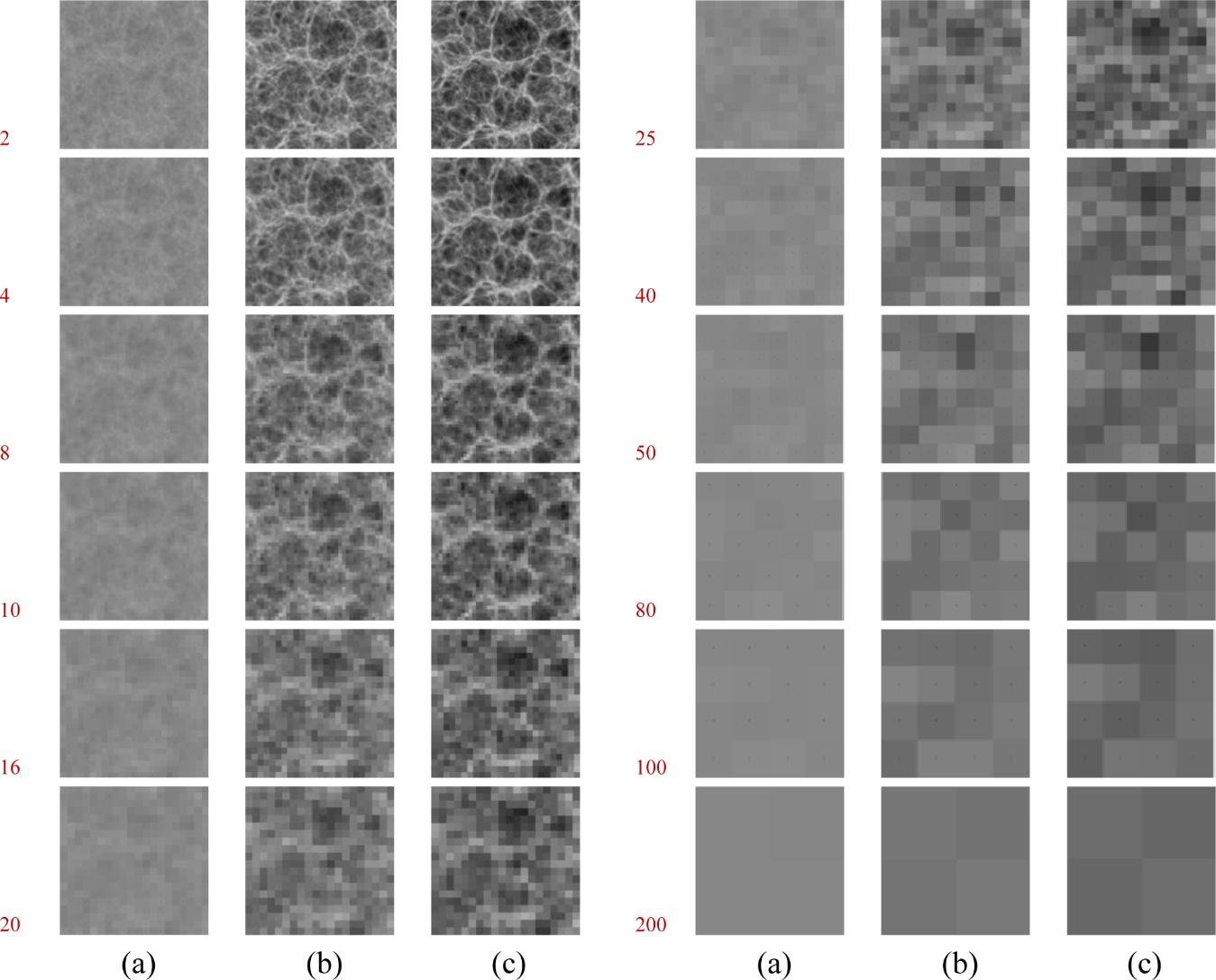
Figure. 7. Example of the stochastic analysis of a 2D picture, in escalating spatial scales, as shown in red colour on the left. The variability of the grouped pixels at different scales are used to construct the climacogram's images; (a), (b) and (c) correspond to different time frames as given in Figure 1.
 |
 |
| (a) | (b) |
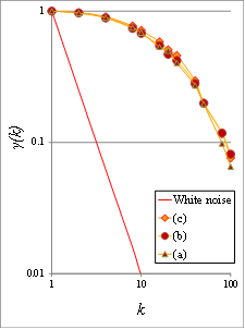
Figure 8. (a) Climacograms of the benchmark images; (b) standardized climacograms of the benchmark images. A standardized climacogram is not helpful to evaluate the range of the evolution of clustering but is helpful to estimate the curves’ slope for further analysis.
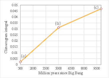
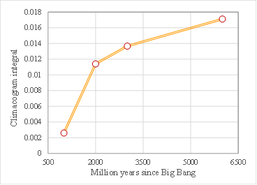
For the integration of all information contained in the 2D climacogram of each timeframe, we evaluate the cumulative areas underneath each climacogram up to the maximum scale (Figure 9a), i.e. the climacogram integral 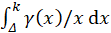
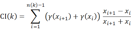
where i is the number of integration intervals up to scale k , xj is the scale j and n(k) is the number of scales up to k. We evaluate CI(k) at the maximum available spatial scale, in order for it to be the best approximation of the limit CI(∞).
In Figure 9b each climacogram is represented by its corresponding integral, permitting the evaluation of the rate of the alteration of clustering through time.
 |
 |
| (a) | (b) |
Figure 9. (a) Cumulative areas underneath each climacogram for each scale; (b) Rate of alteration of clustering through time.
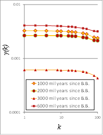
One more example is given in Figures 10 and 11, where we evaluate the evolution of clustering in (randomly picked) zoomed areas from the original images of the evolution of the universe [40] [41].
 |
 |
 |
 |
| (a) | (b) | (c) | (d) |
Figure 10. Example of image analysis, evolution of the universe (zoomed view) [40] [41]: Images of millions of years after the Big Bang (a) 1000; (b) 2000; (c) 3000 (d) 6000
 |
 |
| (a) | (b) |
Figure 11. (a) Climacograms; (b) Rate of alteration of clustering through time.
This method enables the comparison of clustering patterns at various spatial scales and among different time frames, and it is a meaningfull metric for understanding and quantifying the change in clustering through time.
Τhe tool called 2D-C (2D-Climacogram) quantifies the variability of images through the variance of the brightness intensity in grayscale. By a careful selection of images with spatial information, we can quantify how clustering alters over time, which can be useful for either characterizing spatial variability, such as in urbanization, and thus, enabling tracking of their spatio-temporal evolution, or for revealing spatial hidden patterns through scales that may be invisible in the first glance of the image. A range of such applications is presented in [31], with focus in (a) natural sciences, in terms of the evolution of the universe as suggested by cosmological simulations and of the ecosystems, such as forests and lakes, and in (b) social sciences dealing with social structures, as revealed by the evolution of worldwide cropland data, satellite images of night lights and spatial data on urban land cover.
References
- Hurst, H.E.. Long term storage capacities of reservoirs; Trans. Am. Soc. Civil Eng: USA, 1951; pp. 116.
- Mandelbrot B. B. . Fractals: Form, Chance and Dimension; W. H. Freeman and Co.: US, 1977; pp. 365.
- Koutsoyiannis D.; The Hurst phenomenon and fractional Gaussian noise made easy. Hydrological Sciences Journal 2002, 47, 573-595, 10.1080/02626660209492961.
- Koutsoyiannis D.; Dimitriadis P.; Lombardo F.; Stevens S., From fractals to stochastics: Seeking theoretical consistency in analysis of geophysical data, Advances in Nonlinear Geosciences, edited by A.A. Tsonis, 237–278, doi:10.1007/978-3-319-58895-7_14, Springer, 2018.
- Dimitriadis, P. Hurst-Kolmogorov Dynamics in Hydrometeorological Processes and in the Microscale of Turbulence. Ph.D. Thesis, Department of Water Resources and Environmental Engineering—National Technical University of Athens, Athens, Greece, 2017.
- Mandelbrot B.; Van Ness J.W.; Fractional Brownian motions, fractional noises and applications. J. Soc. Ind. Appl. Math.l 1968, 10, 422-437.
- Sargentis G.-F.; Dimitriadis P.; Koutsoyiannis D.; Aesthetical Issues of Leonardo Da Vinci’s and Pablo Picasso’s Paintings with Stochastic Evaluation. Heritage 2020, 3, 283-305, 10.3390/heritage3020017.
- Sargentis G.-F.; Ioannidis R.; Meletopoulos I.T.; Dimitriadis P.; Koutsoyiannis; D. ; Aesthetical issues with stochastic evaluation, European Geosciences Union General Assembly 2020, Geophysical Research Abstracts, Vol. 22, Online, EGU2020- 19832, https://doi.org/10.5194/egusphere-egu2020-19832, European Geosciences Union, 2020.
- Sargentis G.-F.; Dimitriadis P.; Iliopoulou T.; Ioannidis R.; Koutsoyiannis D.; Stochastic investigation of the Hurst-Kolmogorov behaviour in arts, European Geosciences Union General Assembly 2018, Geophysical Research Abstracts, Vol. 20, Vienna, EGU2018-17082, European Geosciences Union, 2018.
- Dimitriadis P.; Koutsoyiannis D.; Tzouka K.; Predictability in dice motion: how does it differ from hydrometeorological processes?. Hydrological Sciences Journal 2016, 61, 1611-1622, 10.1080/02626667.2015.1034128.
- Kolmogorov, A.N.. Wiener spirals and some other interesting curves in a Hilbert space. Selected Works of A. N. Kolmogorov ; Kluwer, Dordrecht, Eds.; Mathematics and Mechanics, Tikhomirov, V. M. : The Netherlands, 1991; pp. 303-307.
- Koutsoyiannis D.; A random walk on water. Hydrology and Earth System Sciences 2010, 14, 585–601.
- Mandelbrot, B. B.; A Fast Fractional Gaussian Noise Generator. Water Resour. Res. 1971, 7(3), 543–553..
- Gneiting T.; Schlather M.; Stochastic Models That Separate Fractal Dimension and the Hurst Effect. SIAM Review 2004, 46, 269-282, 10.1137/s0036144501394387.
- Koutsoyiannis D.; Hurst–Kolmogorov dynamics as a result of extremal entropy production. Physica A: Statistical Mechanics and its Applications 2011, 390, 1424-1432, 10.1016/j.physa.2010.12.035.
- Dimitriadis P.; Koutsoyiannis D.; Stochastic synthesis approximating any process dependence and distribution. Stochastic Environmental Research and Risk Assessment 2018, 32, 1493-1515, 10.1007/s00477-018-1540-2.
- Iliopoulou T.; Koutsoyiannis D.; Revealing hidden persistence in maximum rainfall records. Hydrological Sciences Journal 2019, 64, 1673-1689, 10.1080/02626667.2019.1657578.
- Iliopoulou T.; Koutsoyiannis D.; Projecting the future of rainfall extremes: Better classic than trendy. Journal of Hydrology 2020, 588, 125005, 10.1016/j.jhydrol.2020.125005.
- McGarvey R.; Feenstra J.E.; Mayfield S.; Sautter E. V.; A diver survey method to quantify the clustering of sedentary invertebrates by the scale of spatial autocorrelation. Marine and Freshwater Research 2010, 61, 153-162, 10.1071/mf08289.
- Tachmazidou I.; Verzilli C. J.; De Iorio M.; Genetic Association Mapping via Evolution-Based Clustering of Haplotypes. PLOS Genetics 2007, 3, e111, 10.1371/journal.pgen.0030111.
- Hütt M.-T.; Neff R.; Quantification of spatiotemporal phenomena by means of cellular automata techniques. Physica A: Statistical Mechanics and its Applications 2001, 289, 498-516, 10.1016/s0378-4371(00)00327-7.
- Khater I. M.; Nabi I. R.; Hamarneh G.; A Review of Super-Resolution Single-Molecule Localization Microscopy Cluster Analysis and Quantification Methods. Patterns 2020, 1, 100038, 10.1016/j.patter.2020.100038.
- Murase K.; Kikuchi K.; Miki H.; Shimizu T.; Ikezoe J.; Determination of arterial input function using fuzzy clustering for quantification of cerebral blood flow with dynamic susceptibility contrast-enhanced MR imaging. Journal of Magnetic Resonance Imaging 2001, 13, 797-806, 10.1002/jmri.1111.
- Mier P.; Andrade-Navarro M. A.; FastaHerder2: Four Ways to Research Protein Function and Evolution with Clustering and Clustered Databases. Journal of Computational Biology 2016, 23, 270-278, 10.1089/cmb.2015.0191.
- McDermott P. L.; Wikle C. K.; Bayesian Recurrent Neural Network Models for Forecasting and Quantifying Uncertainty in Spatial-Temporal Data. Entropy 2019, 21, 184, 10.3390/e21020184.
- Beck R.; Dickmann F.; Lovas R. G.; Quantification of the clustering properties of nuclear states. Annals of Physics 1987, 173, 1-29, 10.1016/0003-4916(87)90091-1.
- Abe S.; Suzuki N.; Dynamical evolution of clustering in complex network of earthquakes. The European Physical Journal B 2007, 59, 93-97, 10.1140/epjb/e2007-00259-3.
- Ellam L.; Girolami M.; Pavliotis G. A.; Wilson A.; Stochastic modelling of urban structure. Proceedings of the Royal Society A: Mathematical, Physical and Engineering Sciences 2018, 474, 20170700, 10.1098/rspa.2017.0700.
- Levine N.; Spatial Statistics and GIS: Software Tools to Quantify Spatial Patterns. Journal of the American Planning Association 1996, 62, 381-391, 10.1080/01944369608975702.
- Lee J.; Gangnon R. E.; Zhu J.; Liang J.; Uncertainty of a detected spatial cluster in 1D: quantification and visualization. Stat 2017, 6, 345-359, 10.1002/sta4.161.
- Sargentis G.-F.; Iliopoulou T.; Sigourou S.; Dimitriadis P.; Koutsoyiannis D.; Evolution of Clustering Quantified by a Stochastic Method—Case Studies on Natural and Human Social Structures. Sustainability 2020, 12, 7972, 10.3390/su12197972.
- Koutsoyiannis D.; Hydrology and change. Hydrological Sciences Journal 2013, 58, 1177-1197, 10.1080/02626667.2013.804626.
- Koutsoyiannis D.; Generic and parsimonious stochastic modelling for hydrology and beyond. Hydrological Sciences Journal 2015, 61, 225-244, 10.1080/02626667.2015.1016950.
- Zhang H.; Fritts J. E.;. Goldman S. A.; An entropy-based objective evaluation method for image segmentation, Proc. SPIE 5307, Storage and Retrieval Methods and Applications for Multimedia 2004, (18 December 2003); doi: 10.1117/12.527167
- Koutsoyiannis, D. (2013), Encolpion of stochastics: Fundamentals of stochastic processes, 12 pages, Department of Water Resources and Environmental Engineering – National Technical University of Athens, Athens.
- Koutsoyiannis, D. (2013b), Climacogram-based pseudospectrum: a simple tool to assess scaling properties, European Geosciences Union General Assembly 2013, Geophysical Research Abstracts, Vol. 15, 700 Vienna, EGU2013-4209, European Geosciences Union.
- Dimitriadis P.; Koutsoyiannis D.; Climacogram versus autocovariance and power spectrum in stochastic modelling for Markovian and Hurst–Kolmogorov processes. Stochastic Environmental Research & Risk Assessment 2015, 29, 1649–1669, 10.1007/s00477-015-1023-7, 2015.
- O’Connell, P.E.; Koutsoyiannis, D.; Lins, H.F.; Markonis, Y.; Montanari, A.; Cohn, T.; The scientific legacy of Harold Edwin Hurst . Hydrol. Sci. J., 2016, 61, 1571–1590, 10.1080/02626667.2015.1125998.
- Sargentis G.-F.; Dimitriadis P.; Ioannidis R.; Iliopoulou T.; Koutsoyiannis D.; Stochastic Evaluation of Landscapes Transformed by Renewable Energy Installations and Civil Works. Energies 2019, 12, 2817, 10.3390/en12142817.
- Evolution of the universe . Time machine. Retrieved 2020-10-13
- Di Matteo, T., et al.; Direct cosmological simulations of the growth of black holes and galaxies. . The Astrophysical Journal 2008, 676, 33-53, 10.1086/524921.