Water resources are highly dependent on climatic variations. The quantification of climate change impacts on surface water availability is critical for agriculture production and flood management. The current study focuses on the projected streamflow variations in the transboundary Mangla Dam watershed. Precipitation and temperature changes combined with future water assessment in the watershed are projected by applying multiple downscaling techniques for three periods (2021–2039, 2040–2069, and 2070–2099). Streamflows are simulated by using the Soil and Water Assessment Tool (SWAT) for the outputs of five global circulation models (GCMs) and their ensembles under two representative concentration pathways (RCPs). Spatial and temporal changes in defined future flow indexes, such as base streamflow, average flow, and high streamflow have been investigated in this study. Results depicted an overall increase in average annual flows under RCP 4.5 and RCP 8.5 up until 2099. The maximum values of low flow, median flow, and high flows under RCP 4.5 were found to be 55.96 m3/s, 856.94 m3/s, and 7506.2 m3/s and under RCP 8.5, 63.29 m3/s, 945.26 m3/s, 7569.8 m3/s, respectively, for these ensembles GCMs till 2099. Under RCP 4.5, the maximum increases in maximum temperature (Tmax), minimum temperature (Tmin), precipitation (Pr), and average annual streamflow were estimated as 5.3 °C, 2.0 °C, 128.4%, and 155.52%, respectively, up until 2099. In the case of RCP 8.5, the maximum increase in these hydro-metrological variables was up to 8.9 °C, 8.2 °C, 180.3%, and 181.56%, respectively, up until 2099. The increases in Tmax, Tmin, and Pr using ensemble GCMs under RCP 4.5 were found to be 1.95 °C, 1.68 °C and 93.28% (2021–2039), 1.84 °C, 1.34 °C, and 75.88%(2040–2069), 1.57 °C, 1.27 °C and 72.7% (2070–2099), respectively. Under RCP 8.5, the projected increases in Tmax, Tmin, and Pr using ensemble GCMs were found as 2.26 °C, 2.23 °C and 78.65% (2021–2039), 2.73 °C, 2.53 °C, and 83.79% (2040–2069), 2.80 °C, 2.63 °C and 67.89% (2070–2099), respectively. Three seasons (spring, winter, and autumn) showed a remarkable increase in streamflow, while the summer season showed a decrease in inflows. Based on modeling results, it is expected that the Mangla Watershed will experience more frequent extreme flow events in the future, due to climate change. These results indicate that the study of climate change's impact on the water resources under a suitable downscaling technique is imperative for proper planning and management of the water resources.
Water resources are highly dependent on climatic variations. The quantification of climate change impacts on surface water availability is critical for agriculture production and flood management. The current study focuses on the projected streamflow variations in the transboundary Mangla Dam watershed. Precipitation and temperature changes combined with future water assessment in the watershed are projected by applying multiple downscaling techniques for three periods (2021–2039, 2040–2069, and 2070–2099). Streamflows are simulated by using the Soil and Water Assessment Tool (SWAT) for the outputs of five global circulation models (GCMs) and their ensembles under two representative concentration pathways (RCPs). Spatial and temporal changes in defined future flow indexes, such as base streamflow, average flow, and high streamflow have been investigated in this study. Results depicted an overall increase in average annual flows under RCP 4.5 and RCP 8.5 up until 2099. The maximum values of low flow, median flow, and high flows under RCP 4.5 were found to be 55.96 m3/s, 856.94 m3/s, and 7506.2 m3/s and under RCP 8.5, 63.29 m3/s, 945.26 m3/s, 7569.8 m3/s, respectively, for these ensembles GCMs till 2099. Under RCP 4.5, the maximum increases in maximum temperature (Tmax), minimum temperature (Tmin), precipitation (Pr), and average annual streamflow were estimated as 5.3 °C, 2.0 °C, 128.4%, and 155.52%, respectively, up until 2099. In the case of RCP 8.5, the maximum increase in these hydro-metrological variables was up to 8.9 °C, 8.2 °C, 180.3%, and 181.56%, respectively, up until 2099. The increases in Tmax, Tmin, and Pr using ensemble GCMs under RCP 4.5 were found to be 1.95 °C, 1.68 °C and 93.28% (2021–2039), 1.84 °C, 1.34 °C, and 75.88%(2040–2069), 1.57 °C, 1.27 °C and 72.7% (2070–2099), respectively. Under RCP 8.5, the projected increases in Tmax, Tmin, and Pr using ensemble GCMs were found as 2.26 °C, 2.23 °C and 78.65% (2021–2039), 2.73 °C, 2.53 °C, and 83.79% (2040–2069), 2.80 °C, 2.63 °C and 67.89% (2070–2099), respectively. Three seasons (spring, winter, and autumn) showed a remarkable increase in streamflow, while the summer season showed a decrease in inflows. Based on modeling results, it is expected that the Mangla Watershed will experience more frequent extreme flow events in the future, due to climate change. These results indicate that the study of climate change’s impact on the water resources under a suitable downscaling technique is imperative for proper planning and management of the water resources.
- GCMs
- Mangla Watershed
- Climate Change
- RCPs
- Downscaling
- Bias Correction
- Linear scaling downscaling
- Distribution mapping downscaling
- Change Factor Downscaling
- Future Water Resources of Pakistan
Note:All the information in this draft can be edited by authors. And the entry will be online only after authors edit and submit it.
1. Introduction
Most of the countries in South Asia are observing water stress due to global atmospheric changes. The rising population in urban areas, agriculture, and mismanagement of water resources and climate change has included Pakistan in the countries that are worst affected by climate change [1]. According to a report by the International Monetary Fund (IMF), Pakistan positioned third in the world among the countries prone to severe water scarcity [2]. The International Panel for Climate Change (IPCC) reported a 0.72 °C increase in the total temperature from 1951 to 2012. An expected rise of 1 °C to 3 °C till 2050 and 2 °C to 5 °C is likely to occur until 2100, based on the different greenhouse gases emission scenario. The severe temperature changes affect the land cover and ultimately change the streamflow patterns [3]. Rivers are providing more than fifty percent of the global water requirement [4]. However, river flows are associated with long-term fluctuations in rainfall and temperature, especially in areas where snowmelt is the principal component of the total runoff [5][6][5,6].
General circulation models (GCMs) are widely in use to study future climate change drifts. These models simulate climate variations based on possible projected greenhouse gas emission rates. The spatial resolution of almost all existing GCM models is around 150–300 km, and the spatial resolution of every single GCM alters when comparing with other GCMs [7]. To accurately apprehend the impact of climate change on water resources, the bias correction of the projected results from different climatic models is often performed [8][9][8,9]. Bias correction is beneficial, especially for hydrological modeling studies where streamflow directly connects with precipitation [10][11][12][10–12]. GCMs present large-scale forecasts for several climatic variables [3], but numerous climatic variables are not determined efficiently through the coarser resolution. To overcome this issue, different downscaling techniques are often applied to downscale the projected GCMs data to a fine resolution, but these techniques also provide systematic deviations [13][14][15][13–15]. Many statistical downscaling techniques have been introduced to eliminate systematic deviations [16][17][16,17]. Specific downscaling procedures establish a connection between regional-scale climatic components with the local scale climatic components. By studying the transfer of moisture at a regional scale and air blowing rate, the temperature and precipitation at a local scale can be predicted [18][19][20][21][18–21]. In statistical downscaling techniques, the spatial resolution of the GCMs is not considered, so the calculation of bias correction coefficient must be done effectively by using long period observed and historical climatic data [22][23][22,23]. Multiple studies deal with the drifts of hydro-climatic components of various basins in the upper Indus basin, using several statistical downscaling techniques, and a continuous rise in temperature was projected [24][25][26][27][24–27]. Nevertheless, the temperature is progressing at varying rates in various sub-basins. The history explains numerous rainfall drifts in various sub-basins present in the upper Indus basin [28].
To understand the hydrologic processes and interaction of water balance components under climate change scenarios in Mangla Watershed, the Soil and Water Assessment Tool (SWAT) model is used in this study. SWAT is proficient in modeling a single catchment or a system of hydrologically connected sub-catchments. The GIS-based interface model, ArcSWAT, defines the river network and the point of catchment outflow, and the distribution of sub-catchments and hydrological response units (HRU) [12][29][30][31][32][33][34][35][12,29–35]. The calculation of the time of concentration by SWAT is done by adding overland flow time (time is taken for flow from the remotest point of the sub-basin to reach the water channel) and channel flow time (time taken from upstream channel to the watershed outlet) [36].
The projected climate is significantly affected by the selection of GCMs [35]. In this study, five global circulation models: The Australian Community Climate and Earth-System Simulator version 1 (ACCESS 1.0), Community Climate System Model (CCSM4), Hadley Centre Global Environment Model version 2 (HadGEM2), Max Planck Institute for Meteorology, Earth System Model Low Radiation Emission (MPI-ESM-LR), and Model for Interdisciplinary Research on Climate, Earth System Model (MirocESM), were selected based on their spatial resolution, and two different emission scenarios, RCP4.5, and RCP8.5 were chosen to reproduce future streamflow by applying the hydrological model SWAT (ArcSWAT-2012).
Several studies have defined precipitation and temperature variations as dominating factors that may affect water quantity and quality [37][38][39][37–39] and reported how climate change affects river flows [21][27][40][21,27,40]. Few studies have reported climate change effects on the average annual streamflow in the Mangla Watershed [32][41][32,41], however, the literature on the impact of future climate change on the annual and seasonal base flows and high flows in the watershed is missing. Moreover, investigation of the impact of future climate change on streamflow by considering the elevation band in watersheds is also missing. Previously, only biased corrections of the downscaled GCMs data had been performed without studying the different downscaling techniques.
2. Model Calibration and Validation
2.1. Model Calibration without Considering Elevation Bands
The results of calibration and validation without considering elevation bands in Mangla watershed show a poor model performance, as represented in Figure 14. SWAT model calibration and validation performance evaluation indices, such as p-factor, r-factor, R2, NSE, and PBIAS, did not result in an acceptable range [42][67].
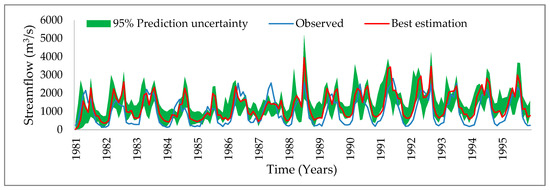
Figure 14. Comparison of simulated flow with the observed flow without considering elevation bands (calibration).
Figure 14 depicts the poor correlation between observed and simulated flows, as these results were simulated without considering elevation bands. The results of calibration without considering elevation bands for p-factor, r-factor, R2, NSE, and PBIAS were 0.43, 1.46, 0.68, 0.46, and −32. The results of the model performance indices, such as p-factor, r-factor, R2, NSE, and PBIAS, show the poor performance of the model in the Mangla Watershed without the use of elevation bands. So, in this research we recommend the hydrological modeling researchers to consider precise elevation bands to obtain accurate simulated results.
2.2. Calibration and Validation Considering Elevation Bands
Calibration and validation results revealed a strong model performance that can be potentially utilized to investigate the impacts of climate change on stream outflows (Figure 25). A strong relationship between model-simulated and observed flows was exhibited, which shows a strong footing of the SWAT model for future flow projections. The values for p-factor, r-factor, R2, NSE, PBIAS are 0.77, 0.99, 0.80, 0.78, and 1.1, respectively. These results show the strong footing of the model for future prediction. The R2 value is 0.80, which shows a strong relationship between the simulated and observed flow. Pbias should be between −20 to +20, and for perfect model footing, it should be close to zero. The pbias value for calibration is closer to the ideal, which is 1.1, which shows a great model performance for future projections. The NSE value in SWAT-CUP results is 0.78, which also represents the accuracy of model calibration.
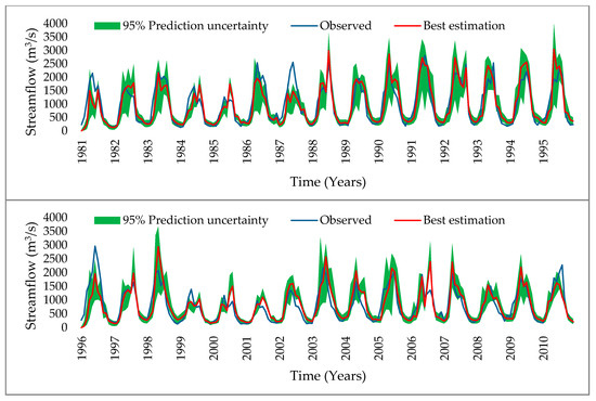
Figure 25. Comparison of simulated flow with observed flow considering elevation bands; calibration (up) and validation (down).
The results of R2, NSE, pbias, p-factor, and r-factor, for calibration and validation, are presented in Table 15. These results depict that the SWAT model performance in the Mangla watershed is very strong [42][67].
Table 15. Results of calibration and validation using the SUFI-2 algorithm.
| Statistical Parameters |
Base Run (Calibration) |
Final Run (Calibration) |
Validation |
| Coefficient of Determination (R2) | 0.28 | 0.80 | 0.77 |
| Bias percentage (Pbias) | 28.46 | 1.1 | −8.2 |
| The efficiency of Nash–Sutcliffe (NSE) | 0.59 | 0.78 | 0.66 |
| Percentage of gauged data wrapped by the simulated 95% uncertainty band (p-factor) | 0.28 | 0.77 | 0.73 |
| Thickness of 95% uncertainty band (r-factor) | 0.47 | 0.95 | 0.96 |
The initial values of some parameters, such as curve number 2 for soil conservation services (CN2), the alpha factor for base flow in bank storage (days) (ALPHA_BF), delay in groundwater in days (GW_DELAY), the minimum depth of water in the shallow aquifer essential for backflow (mm) GWQMN, and groundwater revap coefficient (GW_REVAP), were taken from the literature [30]. The parameters used during the model calibration are shown in Table 6. The northern part of the Mangla Watershed is a partially snow-covered region [32] so some snow cover parameters, such as the temperature of snowfall (SFTM), the Base temperature of snowmelt (SMTMP), the maximum rate of snowmelt over a year (SMFMX), the minimum rate of snowmelt over a year (SMFMN), the minimum amount of snow water resembles 100% of snow cover (SNOCOVMX), and the volume of snow that corresponds to 50% of snow cover (SNO50COV), were also utilized. The minimum initial value given to SFTM is −5 and the maximum value given is 5. The parameter SNOCOVMX was initially set between 0 and 400, whereas the minimum and maximum values designated to SNO50COV were 0.1 and 0.6. More details about these parameters can be found in the user manual of SWAT-CUP_2012 [43][70].
Table 6. Explanation of sensitive parameters, along with their initial and adopted values.
| Rank | Parameter | Description | Initial Range | Calibrated Value | Sensitivity Analysis | ||
|
Min |
Max |
p-Values |
T-Stat | ||||
| 1 | CN2 | Curve number 2 for soil conservation services | −0.4 | 0.2 | 0.09 | 1.75E-07 | −5.69 |
| 2 | ALPHA_BF | The alpha factor for base flow in bank storage (days) | 0 | 0.6 | 0.5 | 0.659 | −0.44 |
| 3 | GW_DELAY | Delay in groundwater in days | 90 | 200 | 118.05 | 0.124 | −1.54 |
| 4 | GWQMN | Minimum depth of water in the shallow aquifer essential for backflow (mm) | 0 | 500 | 1.56 | 0.805 | −0.25 |
| 5 | GW_REVAP | Groundwater revap coefficient | 0 | 0.2 | 0.16 | 0.939 | 0.08 |
| 6 | RCHRG_DP | Deep percolation into the aquifer | 0 | 1 | 0.37 | 0.243 | −1.17 |
| 7 | CH_N2 | Main channel’s manning (n) value | 0 | 0.3 | 0.11 | 0.086 | 1.72 |
| 8 | CH_K2 | Main channel’s effective hydraulic conductivity | 5 | 100 | 77.53 | 0.954 | −0.06 |
| 9 | ALPHA_BNK | Bank storage base flow’s alpha factor (day) | 0 | 1 | 0.98 | 0.283 | 1.08 |
| 10 | SOL_AWC | Soil available water capacity | −0.2 | 0.4 | 0.14 | 0.482 | −0.7 |
| 11 | SOL_K | Hydraulic conductivity of saturated soil | −0.8 | 0.8 | 0.48 | 0.111 | −1.6 |
| 12 | SOL_BD | Bulk density of moist soil | 0 | 1 | 0.87 | 0.419 | −0.81 |
| 13 | SMFMX | The maximum rate of snowmelt over a year | 0 | 20 | 5.61 | 1.83E-08 | 8.87 |
| 14 | SMFMN | The minimum rate of snowmelt over a year | 0 | 20 | 3.19 | 0.06 | −1.88 |
| 15 | SMTMP | Base temperature of snowmelt (°C) | −5 | 5 | 3.49 | 0.489 | 0.69 |
| 16 | SFTMP | The temperature of snowfall (°C) | −5 | 5 | −2.15 | 2.48E-08 | 8.53 |
| 17 | TIMP | Temperature lag factor for snowpack | 0 | 1 | 0.32 | 0.845 | −0.2 |
| 18 | TLAPS | Lapse rate of temperature | −20 | 20 | −5.05 | 2.51E-06 | −5.19 |
| 19 | PLAPS | Lapse rate of precipitation | −300 | 300 | 117.86 | 0.015 | −2.43 |
| 20 | ESCO | Soil evaporation compensation factor | 0 | 1 | 0.68 | 0.436 | −0.78 |
| 21 | SNOCOVMX | The minimum amount of snow water resembles 100% of snow cover (mm) | 0 | 400 | 302.76 | 0.38 | −0.88 |
| 22 | SNO50COV | The volume of snow that corresponds to 50% of snow cover | 0.1 | 0.6 | 0.49 | 0.939 | −0.08 |
3. Performance Evaluation of The SWAT Model in Terms of Low and High Flows
The simulated low streamflow and high streamflow by the SWAT model were compared with observed low stream flows and observed high streamflow, respectively. The results indicated a strong correlation coefficient of 0.94 and 0.98 for low and high streamflow, respectively. The values of the coefficient of determination (R2) also indicated that the SWAT model performed well in simulating low and high streamflow. The R2 values were 0.88 and 0.96 for low streamflow and high streamflow respectively. Figure 36 shows the comparison between observed and simulated low streamflow and observed and simulated high streamflow. The values of the coefficient of determination (R2) also represent that the observed and simulated low flows and observed and simulated high flows have a strong relationship. These indices depict that the SWAT model is performing well in simulating low flows and high flows.
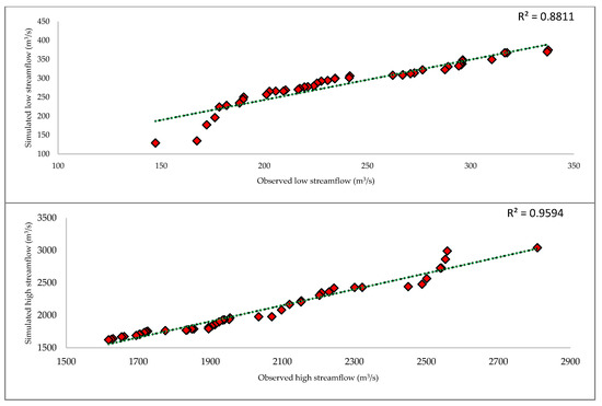
Figure 36. Comparison of observed and simulated low streamflow (up) and observed and simulated high streamflow (down).
4. Seasonal Change in Temperature and Precipitation
The variation in mean seasonal rainfall is limited in spring and winter while shifting in rainfall is more during autumn and summer seasons for five GCMs. The rainfall during the moon-soon season is predicted to be more intense, while there will be a large increase in temperature; up to 8.4 °C. From Figure 47, it is concluded that in the 20th century the temperature is relatively less than in the 21st century; meanwhile, the temperature is increasing at a relatively steeper rate as compared with the previous period. In the year 1990, the average temperature of the whole watershed was 24.5 °C, whereas the expected average annual temperature for the 2030 scenario is 26.2 °C. It can be observed that there is almost a 1.7 °C increase in temperature in four decades. However, it can also be observed that in 2070, the average temperature will reach 29.54 °C, as there will be a rise of almost 3.34 °C in the next four decades. For 2100, the temperature will touch 32.08 °C, from which it can be observed that the temperature will rise to 2.54 °C during the period from 2070 to 2100. Considering RCP (4.5), it can be observed that temperature will tend to rise at a higher rate during the middle of the century, as compared to the end of the century.
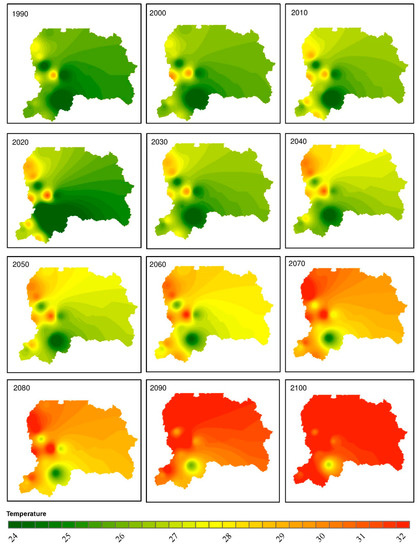
Figure 47. The projected change in average temperature (°C) from 1990 to 2100.
Figure 47 revealed the average temperature from 1990 to 2100 within the transboundary Mangla Watershed. The best adopted downscaling technique for the watershed, i.e., distribution mapping downscaling, was used to predict these results. Figure 47 represents that the maximum rise in temperature till 2100 will be 8.9 °C. It is a large increase in temperature which will definitely increase evapotranspiration and also cause glaciers to melt and will severely affect freshwater resources in the future.
Figure 58 shows the projected change in precipitation (mm) over the Mangla watershed from the year 1990 to 2100. In 1990, there was less precipitation in most of the watershed, and it increases continuously in the future from 2021 to 2100. The northern part of the Mangla Watershed located at a higher altitude registered more rainfall as compared to the southern part of the watershed. In the late century, there will be more precipitation due to an increase in temperature. The increase in temperature ultimately causes evapotranspiration and precipitation to surge.
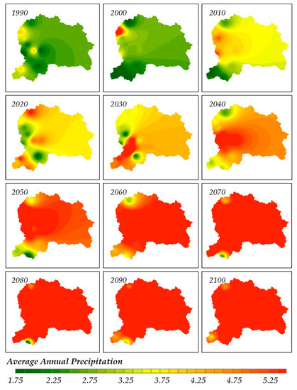
Figure 58. The projected change in average annual rainfall (mm) from 1990 to 2100.
Figure 69 (a) shows the average annual precipitation of ensembled GCM models [44][71] from 1981 to 2010 under three downscaling techniques for the RCP 4.5 radiative forcing emission scenario. The average annual precipitation under change factor downscaling ranges from 3.2 mm to 5.5 mm. The average annual precipitation from ensembled model output ranges from 2.78 mm to 4.89 mm under distribution mapping downscaling, and 2.54 mm to 9.4 mm under linear scaling. Figure 9 (b) shows the GCMs ensembled average annual precipitation under RCP 8.5. The change factor downscaling ranges between 3.14 mm and 5.47 mm, distribution mapping ranges from 2.44 mm to 4.65 mm, and linear scaling ranges between 2.87 mm and 9.33 mm.
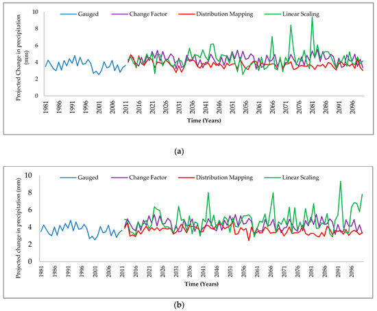
Figure 69. GCMs model ensembled average annual precipitation change from 1981 to 2100 under three downscaling techniques. (a) RCP 4.5, (b) RCP 8.5.
Figure 710 shows the GCMs ensembled average temperature trends from 1981 to 2100. The temperature under both RCPs showed an increasing trend. Figure 710 (a) shows the change in Tmax and Tmin from 1981 to 2100 under the RCP 4.5 scenario. The increase in Tmax under change factor (CF) downscaling is 6.32 °C and an increase in Tmin is 5.45 °C. There is a 5.36 °C rise in Tmax and 4.34°C in Tmin under the distribution mapping downscaling technique. In linear scaling, there is a 3.92°C increase in Tmax and 2.78 °C in Tmin. Figure 710 (b) shows the change in Tmax and Tmin under the RCP 8.5 scenario. The Tmax and Tmin were increased by 7.89 °C and 6.85 °C respectively under change factor downscaling and RCP 8.5. In distribution mapping, the Tmax was increased by 7.79 °C, whereas the Tmin was increased by 7.74°C under RCP 8.5. The linear scaling downscaling has an increase of Tmax of 5.99°C and a Tmin of 5.37 °C.
Figure 710. GCMs ensembled average temperature from 1981 to 2100 under three downscaling techniques; (a) RCP 4.5, (b) RCP 8.5.
References
- Scott, D.; Hall, C.M.; Gössling, S. A review of the IPCC Fifth Assessment and implications for tourism sector climate resilience and decarbonization. Sustain. Tour. 2016, 24, 8–30, doi:10.1080/09669582.2015.1062021.
- Hussain Sargana, M.; Saud, M. Pakistan’s Internal Security Dynamics: Way Forward. Peace, Dev. Commun. 2019, 3, 1–26.
- Stocker, T.F.; Qin, D.; Plattner, G.K.; Tignor, M.M.B.; Allen, S.K.; Boschung, J.; Nauels, A.; Xia, Y.; Bex, V.; Midgley, M. Climate change 2013 the physical science basis: Working Group I contribution to the fifth assessment report of the intergovernmental panel on climate change; Cambridge University Press, UK, 2013.
- Bolch, T. Hydrology: Asian glaciers are a reliable water source. Nature 2017, 545, 161–162.
- Lutz, A.F.; Immerzeel, W.W.; Shrestha, A.B.; Bierkens, M.F.P. Consistent increase in High Asia’s runoff due to increasing glacier melt and precipitation. Clim. Chang. 2014, 4, 587–592, doi:10.1038/nclimate2237.
- Deng, H.; Chen, Y.; Wang, H.; Zhang, S. Climate change with elevation and its potential impact on water resources in the Tianshan Mountains, Central Asia. Planet. Change 2015, 135, 28–37, doi:10.1016/j.gloplacha.2015.09.015.
- Taylor, K.E.; Stouffer, R.J.; Meehl, G.A. An overview of CMIP5 and the experiment design. Am. Meteorol. Soc. 2012, 93, 485–498.
- Muerth, M.J.; Gauvin St-Denis, B.; Ricard, S.; Velázquez, J.A.; Schmid, J.; Minville, M.; Caya, D.; Chaumont, D.; Ludwig, R.; Turcotte, R. On the need for bias correction in regional climate scenarios to assess climate change impacts on river runoff. Earth Syst. Sci. 2013, 17, 1189–1204, doi:10.5194/hess-17-1189-2013.
- Teng, J.; Potter, N.J.; Chiew, F.H.S.; Zhang, L.; Wang, B.; Vaze, J.; Evans, J.P. How does bias correction of regional climate model precipitation affect modelled runoff? Earth Syst. Sci. 2015, 19, 711–728, doi:10.5194/hess-19-711-2015.
- Christensen, J.H.; Boberg, F.; Christensen, O.B.; Lucas-Picher, P. On the need for bias correction of regional climate change projections of temperature and precipitation. Res. Lett. 2008, 35, doi:10.1029/2008GL035694.
- Maurer, E.P.; Hidalgo, H.G. Utility of daily vs. monthly large-scale climate data: An intercomparison of two statistical downscaling methods. Earth Syst. Sci. 2008, 12, 551–563, doi:10.5194/hess-12-551-2008.
- Mbaye, M.L.; Haensler, A.; Hagemann, S.; Gaye, A.T.; Moseley, C.; Afouda, A. Impact of statistical bias correction on the projected climate change signals of the regional climate model REMO over the Senegal River Basin. J. Climatol. 2016, 36, 2035–2049, doi:10.1002/joc.4478.
- Fowler, H.J.; Blenkinsop, S.; Tebaldi, C. Linking climate change modelling to impacts studies: Recent advances in downscaling techniques for hydrological modelling. J. Climatol. 2007, 27, 1547–1578.
- Di Luca, A.; de Elía, R.; Laprise, R. Potential for small scale added value of RCM’s downscaled climate change signal. Dyn. 2013, 40, 601–618, doi:10.1007/s00382-012-1415-z.
- Kotlarski, S.; Keuler, K.; Christensen, O.B.; Colette, A.; Déqué, M.; Gobiet, A.; Goergen, K.; Jacob, D.; Lüthi, D.; Van Meijgaard, E.; et al. Regional climate modeling on European scales: a joint standard evaluation of the EURO-CORDEX RCM ensemble. Model Dev. 2014, 7, 1297–1333, doi:10.5194/gmd-7-1297-2014.
- Gellens, D.; Roulin, E. Streamflow response of Belgian catchments to IPCC climate change scenarios. Hydrol. 1998, 210, 242–258, doi:10.1016/S0022-1694(98)00192-9.
- Chen, J.; Brissette, F.P.; Chaumont, D.; Braun, M. Performance and uncertainty evaluation of empirical downscaling methods in quantifying the climate change impacts on hydrology over two North American river basins. Hydrol. 2013, 479, 200–214, doi:10.1016/j.hydrol.2012.11.062.
- Pervez, M.S.; Henebry, G.M. Assessing the impacts of climate and land use and land cover change on the freshwater availability in the Brahmaputra River basin. Hydrol. Reg. Stud. 2015, 3, 285–311, doi:10.1016/j.ejrh.2014.09.003.
- Zhang, Y.; You, Q.; Chen, C.; Ge, J. Impacts of climate change on streamflows under RCP scenarios: A case study in Xin River Basin, China. Res. 2016, 178–179, 521–534, doi:10.1016/j.atmosres.2016.04.018.
- Wilby, R.L.; Dawson, C.W.; Barrow, E.M. SDSM - A decision support tool for the assessment of regional climate change impacts. Model. Softw. 2002, 17, 145–157, doi:10.1016/s1364-8152(01)00060-3.
- Mahmood, R.; Babel, M.S. Evaluation of SDSM developed by annual and monthly sub-models for downscaling temperature and precipitation in the Jhelum basin, Pakistan and India. Appl. Climatol. 2013, 113, 27–44, doi:10.1007/s00704-012-0765-0.
- Maraun, D.; Wetterhall, F.; Ireson, A.M.; Chandler, R.E.; Kendon, E.J.; Widmann, M.; Brienen, S.; Rust, H.W.; Sauter, T.; Themel, M.; et al. Precipitation downscaling under climate change: Recent developments to bridge the gap between dynamical models and the end user. Geophys. 2010, 48, 32–41, doi:10.1029/2009RG000314.
- Sachindra, D.A.; Perera, B.J.C. Statistical downscaling of general circulation model outputs to precipitation accounting for non-stationarities in predictor-predictand relationships. PLoS ONE 2016, 11, 67–78, doi:10.1371/journal.pone.0168701.
- Garee, K.; Chen, X.; Bao, A.; Wang, Y.; Meng, F. Hydrological modeling of the upper indus basin: A case study from a high-altitude glacierized catchment Hunza. Water 2017, 9, 40–60, doi:10.3390/w9010017.
- Tahir, A.A.; Adamowski, J.F.; Chevallier, P.; Haq, A.U.; Terzago, S. Comparative assessment of spatiotemporal snow cover changes and hydrological behavior of the Gilgit, Astore and Hunza River basins (Hindukush–Karakoram–Himalaya region, Pakistan). Atmos. Phys. 2016, 128, 793–811, doi:10.1007/s00703-016-0440-6.
- Ul Hasson, S.; Böhner, J.; Lucarini, V. Prevailing climatic trends and runoff response from Hindukush-Karakoram-Himalaya, upper Indus Basin. Earth Syst. Dyn. 2017, 8, 337–355, doi:10.5194/esd-8-337-2017.
- DR, A.; HJ, F. Erratum to: Using meteorological data to forecast seasonal runoff on the River Jhelum, Pakistan. J. Hydrol. 2009, 364, 200–229, doi:10.1016/j.jhydrol.2008.11.004.
- Amin, A.; Nasim, W.; Mubeen, M.; Sarwar, S.; Urich, P.; Ahmad, A.; Wajid, A.; Khaliq, T.; Rasul, F.; Hammad, H.M.; et al. Regional climate assessment of precipitation and temperature in Southern Punjab (Pakistan) using SimCLIM climate model for different temporal scales. Appl. Climatol. 2018, 131, 121–131, doi:10.1007/s00704-016-1960-1.
- Zaman, M.; Fang, G.; Mehmood, K.; Saifullah, M. Trend change study of climate variables in Xin’anjiang-Fuchunjiang watershed, China. Meteorol. 2015, 1–13, doi:10.1155/2015/507936.
- Adnan, M.; Kang, S. change; Zhang, G. shuai; Anjum, M.N.; Zaman, M.; Zhang, Y. qing Evaluation of SWAT Model performance on glaciated and non-glaciated subbasins of Nam Co Lake, Southern Tibetan Plateau, China. Mt. Sci. 2019, 16, 1075–1097, doi:10.1007/s11629-018-5070-7.
- Zaman, M.; Naveed Anjum, M.; Usman, M.; Ahmad, I.; Saifullah, M.; Yuan, S.; Liu, S. Enumerating the Effects of Climate Change on Water Resources Using GCM Scenarios at the Xin’anjiang Watershed, China. Water. 2018, 10, 1296–1305, doi:10.3390/w10101296.
- Babur, M.; Babel, M.S.; Shrestha, S.; Kawasaki, A.; Tripathi, N.K. Assessment of climate change impact on reservoir inflows using multi climate-models under RCPs-the case of Mangla Dam in Pakistan. Water. 2016, 8, 1–11, doi:10.3390/w8090389.
- Olsson, T.; Jakkila, J.; Veijalainen, N.; Backman, L.; Kaurola, J.; Vehviläinen, B. Impacts of climate change on temperature, precipitation and hydrology in Finland-studies using bias corrected Regional Climate Model data. Earth Syst. Sci. 2015, 19, 3217–3238, doi:10.5194/hess-19-3217-2015.
- Tschöke, G.V.; Kruk, N.S.; de Queiroz, P.I.B.; Chou, S.C.; de Sousa Junior, W.C. Comparison of two bias correction methods for precipitation simulated with a regional climate model. Appl. Climatol. 2017, 127, 841–852, doi:10.1007/s00704-015-1671-z.
- Arnell, N. Effects of IPCC SRES* emissions scenarios on river runoff: A global perspective. Earth Syst. Sci. 2003, 7, 619–641.
- Neitsch, S.L.; Arnold, J.G.; Kiniry, J.R.; Williams, J.R. Soil and Water Assessment Tool Theoretical Documentation Version 2005; Blackland Research Center: Temple, TX, USA, 2005.
- Mehdi, B.; Ludwig, R.; Lehner, B. Evaluating the impacts of climate change and crop land use change on streamflow, nitrates and phosphorus: A modeling study in Bavaria. Hydrol. Reg. Stud. 2015, 4, 60–90, doi:10.1016/j.ejrh.2015.04.009.
- Pulido-Velazquez, M.; Peña-Haro, S.; García-Prats, A.; Mocholi-Almudever, A.F.; Henríquez-Dole, L.; Macian-Sorribes, H.; Lopez-Nicolas, A. Integrated assessment of the impact of climate and land use changes on groundwater quantity and quality in the Mancha Oriental system (Spain). Earth Syst. Sci. 2015, 19, 1677–1693.
- Shrestha, S.; Shrestha, M.; Babel, M.S. Modelling the potential impacts of climate change on hydrology and water resources in the Indrawati River Basin, Nepal. Earth Sci. 2016, 75, 1–13, doi:10.1007/s12665-015-5150-8.
- Mall, R.K.; Gupta, A.; Singh, R.; Singh, R.S.; Rathore, L.S. Water resources and climate change: An Indian perspective. Sci. 2006, 90, 1610–1626.
- Mahmood, R.; Jia, S. Assessment of Impacts of Climate Change on the Water Resources of the Transboundary Jhelum River Basin of Pakistan and India. Water 2016, doi:10.3390/w8060246.