Flowback-produced water (FP) is a waste fluid associated with hydraulic fracturing in unconventional oil and gas development (UOG). Initially, FP reflects the composition of the hydraulic fracturing fluid, which is referred as flowback water (FBW). After the initial months of well production, the waste fluid is predominantly representative of the formation and is known as produced water (PW).
- produced water
- hydraulic fracturing
1. Technologies Utilized in Produced Water Treament
| Bakken Shale Range (mg/L) [9][14][15][16][17][18] |
Permian Basin Range (mg/L) [19][20][21] |
Well Stimulation (mg/L) [11] |
Agricultural Use (mg/L) (EPA) |
Drinking Water (mg/L) (FAO & EPA) |
||||||
|---|---|---|---|---|---|---|---|---|---|---|
| METAL | ||||||||||
| Magnesium (Mg) | 1530–3790 | 1630–1950 | 2000 | |||||||
| Iron (Fe) | 0.70–30.20 | 11 | 10.00 | 5.00 | 0.30 | |||||
| Manganese (Mn) | 5.20–17.20 | 11.00–53.00 | 0.20 | 0.05 | ||||||
| Aluminium (Al) | <LOQ–8.30 | USD/year | 5.00 | $171,730,000 | $831,605,0000.05–0.20 | |||||
| Calcium (Ca) | 13,140–41,160 | 10,000–15,000 | 2000 | |||||||
| Water management Cost—Scenario 1 | USD/year | $377.30 M | $1.76 B | Sodium (Na) | 89,100–189,000 | 48,000–54,000 | 69.00 | |||
| Treatment and reuse | Potassium (K) | 3510–9530 | 570–1100 | |||||||
| Chemical oxidation | USD/bbl | $0.20 | $0.20 | (Correspondence w/water treatment company) | Barium (Ba) | 6.40–26.30 | 0.00–16.00 | 20.00 | 2.00 | |
| Chemical precipitation & nanofiltration | USD/bbl | $0.24 | $0.24 | Strontium (Sr) | 709–2450 | 730.0–820.0 | ||||
| Cobalt (Co) | 0.030–0.20 | N/A | 0.050 | |||||||
| Nickel (Ni) | <LOQ–3.80 | 0.020 | 0.20 | 0.07 | ||||||
| Lithium (Li) | 34.50–89.70 | 18.80 | 2.50 | |||||||
| Chromium (Cr) | 0.10 | 0.10 | ||||||||
| Radium 226 (Ra) | 527.1–1211 pCi/L | 5.000 pCi/L | ||||||||
| Uranium (U) | 30.00 µg/L | |||||||||
| Copper (Cu) | 4.60–16.90 | 0.20 | 1.00 | |||||||
| Zinc (Zn) | 2.50–10.10 | 2.00 | 5.00 | |||||||
| Arsenic (As) | 1.1 | 0.10 | 0.01 | |||||||
| Beryllium (Be) | 0.10 | 0.004 | ||||||||
| Lead (Pb) | 0.00–3.50 | 5.00 | 0.015 | |||||||
| Silver (Ag) | 0.10 | |||||||||
| Molybdenum (Mo) | 0.01 | |||||||||
| Cadmium (Cd) | 0.001–0.031 | 0.01 | 0.005 | |||||||
| Vanadium (V) | 0.60–1.00 | 0.10 | ||||||||
| Thallium (Tl) | 0.00–0.20 | 0.002 | ||||||||
| Antimony (Sb) | 0.006 | |||||||||
| Rubidium (Rb) | 0.30–12.90 | |||||||||
| Mercury (Hg) | 0.002 | |||||||||
| NON-METAL | ||||||||||
| Chloride (Cl−) | 21,728–136,220 | 111,000–138,000 | 30,000–50,000 | 92.00 | 250.0 | |||||
| Bromide (Br−) | 91.6–558 | 1370–1650 | ||||||||
| Silicon (Si) | 32 | 35.00 | ||||||||
| Fluoride (F−) | 1.00 | 4.00 | ||||||||
| Boron (B) | 25.0–260.1 | 10.00 | 0.70 | |||||||
| Selenium (Se) | 0.10–1.00 | 0.02 | 0.05 | |||||||
| POLYATOMIC IONS | ||||||||||
| Sulfate SO42−) | 0.000–293.0 | 515–743 | 500 | 250 | ||||||
| Bicarbonate (HCO3−) | 35.00–856.0 | 92–160 | 300 | 91.50 | ||||||
| Nitrite (NO2−) | 1.00 | |||||||||
| Nitrate (NO3−) | 5.000 | 10.00 | ||||||||
| Phosphate (PO43) | 584 * | |||||||||
| Ammonium (NH4+) | 44.8–2520 | 655 | ||||||||
| Cyanide (CN−) | 0.200 | |||||||||
| OTHER PARAMETERS | ||||||||||
| pH | 4.1–7.2 | 7.30 | 6.0–8.0 | 6.5–8.4 | 6.5–8.5 | |||||
| TDS | 128,300–388,600 | 174,213–212,984 | 450 | 500 | ||||||
| TSS | 7040 * | 6850–21,820 | 500 | |||||||
| Total nitrogen | ||||||||||
| TOC | 311 * | 86.25–184.21 | ||||||||
| Alkalinity (CaCO3) | 0–562.8 | 2345 | ||||||||
| Turbidity (NTU) | 13 | 53.4 | ||||||||
| DOC | 80 * | 63.45–145.71 | ||||||||
| Conductivity (mS/cm) | 201.2 | |||||||||
| Nonvolatile dissolved organic carbon (NVDOC) | 1.13–3.31 | |||||||||
| Total Hardness(mg/L CaCO3) | 31,000–59,000 | |||||||||
| Chemical Oxygen demand (COD) | 20,000–79,000 | |||||||||
2. Adsorption is applied for the sequestration of organics and metal contaminants. However, it is more of a polishing step for other preceding treatment modalities instead of being a sole separation technique on its own. It is important to note that the adsorption efficiency of various media is mediated by salinity. Activated carbon media are effective for organic contaminants, whereas, activated zeolite is an effective adsorbent for the removal of scaling ions such as Ca2+ and Mg2+ [60] [22] that are generally present in elevated concentrations in FP (see Table 1). Other possible absorbents include alumina and organoclays [8][4]. In recent studies, Sun et al. achieved the removal of several metal pollutants; for instance, Cu(ll), As(V), Cr (Vl), Cr(ll) and Zn(ll) on Fe-impregnated biochar, a carbon-rich fine-grained pyrolysis residue [23][61].
3. Membrane filtration consists of the separation of a fluid from dissolved substances by a porous surface. This includes reverse osmosis (RO), microfiltration (MF), nanofiltration (NF), ultrafiltration (UF) and forward osmosis (FO). RO removes solids by the application of hydraulic pressure to move water molecules through a semi-permeable membrane; MF allows the physical separation of suspended solids and turbidity depletion via the retention of particles larger than the micropores in the membranes. UF reduces odor, organic matter and color with pore membranes on the order of microns. NF offers selective particle rejection based on size and charge, which lessens multivalent ions, and FO lowers TDS in high-saline brines, benefiting from osmotic pressure and transporting water molecules through a semipermeable membrane from the less-concentrated feed to the highly concentrated solution [22]. Some modalities could be applied as treatment technologies on their own, such as MF and UF; others are steps in a more complex separation process. The obstacles to overcome include the membrane fooling/clogging due to interactions with VOCs in NF/RO, fouling caused by high Fe concentration in MF/UF, and scaling in RO [8][9][23][24] as well as RO’s limitation to ionic strengths lower than that of sea water (approx. 40,000 ppm) [25].
4. Electrocoagulation (EC) promotes the precipitation of metals in the form of hydroxides by the addition of direct current through a metal electrode. This has been shown to be efficient and economically feasible for wastewater [26]. Previous studies have demonstrated high removals of turbidity, COD, oils and greases by EC. For example, Kausley et al. reported efficacy in the removal of total organic carbon (TOC) and scaling-causing ions, particularly Ca2+, Mg2+, CO32− and HCO3-, from synthetic PW and PW [26][27]. The precipitation of metal cations in the form of hydroxides could be further exploited to make the treatment of FP more economically viable to the industrial sector through the generation and commercialization of Cu2+, Mn2+, Zn2+, Al3+, Fe3+, Ni2+, Mg2+, Ca2+, Na+ and several other metal hydroxides. Moreover, HCl could be produced by hydrolysis of Cl2 gas generated during the process [27][28][29][30]. (Greater details will be discussed in subsequent sections of this review).
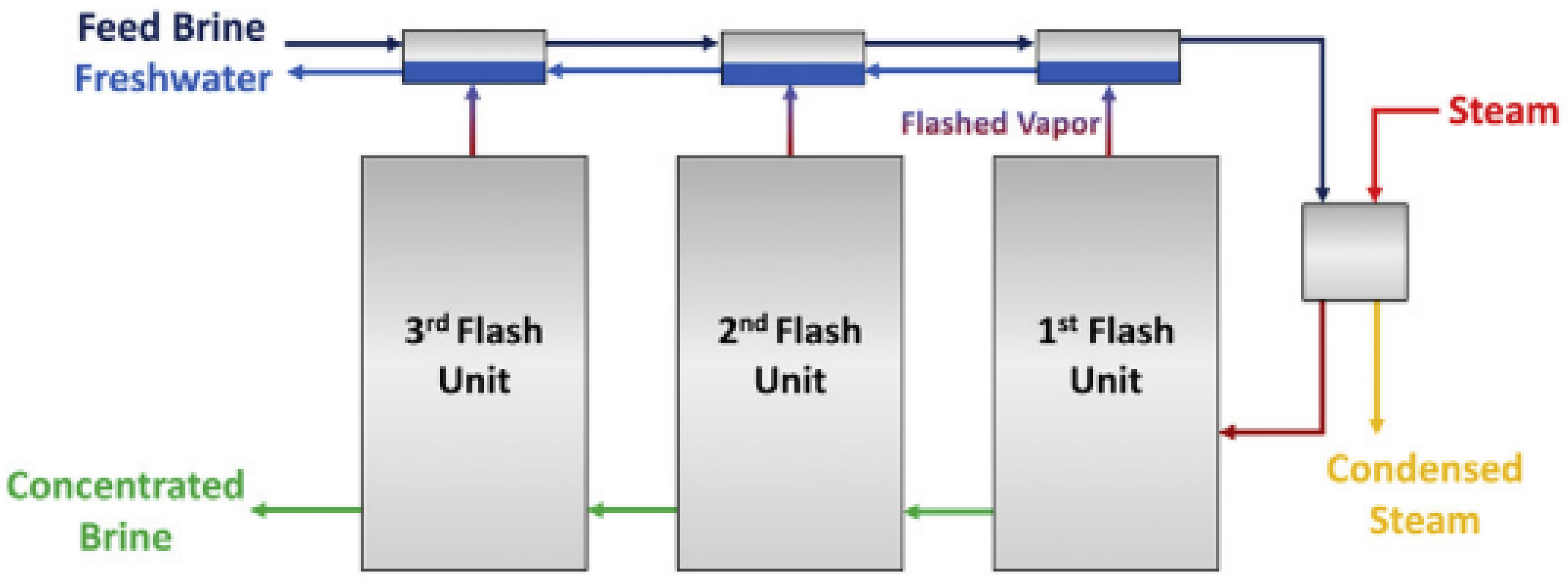
5. Distillation is a thermal process in which solid particles are separated from liquid matrix by boiling point differences. One of the promising variations for brine desalination is multistage flash distillation (MSF). In MSF, the saline solution is converted into a vapor state and then goes through successive units in which the solution evaporates and condensates. In each unit, a fraction of the original feed remains as a highly concentrated brine (see Figure 1) [22]. The technique produces high-quality fresh water [31] and is efficient in the treatment of brackish/sea water. Nevertheless, for future applications in PW treatment, it is suggested to pretreat the inlet water with chemical softeners, filtrations and/or ion exchange technologies to avoid scaling and fouling, as well as to upgrade the infrastructure material to stainless steel to prevent corrosion [22]. The latter increases capital costs. Additionally, the salts produced by this treatment modality can serve as a feedstock for electrocatalytic processes to produce acids (HCl) and caustic agents (NaOH).
2. Costs Associated with Produced Water Treatment
| Unit | Bakken Region | Permian Region | Reference | |
|---|---|---|---|---|
| Saltwater Disposal (SWD) cost | ||||
| Disposal volume | bbl/year | 3.43 × 10⁸ | 1.6 × 10⁹ | [41][51] |
| Transportation Cost * | USD/bbl | $0.60 | $0.60 | [47] |
| Well Injection Cost | USD/bbl | $0.5 | $0.5 | [52] |
| Well disposal Cost | ||||
| (Correspondence w/water treatment company) | ||||
| Water management Cost—Scenario 2 | ||||
| USD/year | $150.92 M | $704.00 M | ||
References
- Rosenblum, J.; Nelson, A.W.; Ruyle, B.; Schultz, M.; Ryan, J.N.; Linden, K.G. Temporal characterization of flowback and produced water quality from a hydraulically fractured oil and gas well. Sci. Total Environ. 2017, 596–597, 369–377.
- Oetjen, K.; Chan, K.E.; Gulmark, K.; Christensen, J.H.; Blotevogel, J.; Borch, T.; Spear, J.R.; Cath, T.Y.; Higgins, C.P. Temporal characterization and statistical analysis of flowback and produced waters and their potential for reuse. Sci. Total Environ. 2018, 619–620, 654–664.
- Ferrer, I.; Thurman, E.M. Chemical constituents and analytical approaches for hydraulic fracturing waters. Trends Environ. Anal. Chem. 2015, 5, 18–25.
- Stringfellow, W.T.; Domen, J.K.; Camarillo, M.K.; Sandelin, W.L.; Borglin, S. Physical, chemical, and biological characteristics of compounds used in hydraulic fracturing. J. Hazard. Mater. 2014, 275, 37–54.
- Hildenbrand, Z.L.; Santos, I.; Liden, T.; Carlton, D.D.; Varona-Torres, E.; Martin, M.S.; Reyes, M.L.; Mulla, S.R.; Schug, K.A. Characterizing variable biogeochemical changes during the treatment of produced oilfield waste. Sci. Total Environ. 2018, 634, 1519–1529.
- Khalil, C.A.; Prince, V.L.; Prince, R.C.; Greer, C.W.; Lee, K.; Zhang, B.; Boufadel, M.C. Occurrence and biodegradation of hydrocarbons at high salinities. Sci. Total Environ. 2021, 762, 143165.
- Mauter, M.S.; Palmer, V.R. Expert Elicitation of Trends in Marcellus Oil and Gas Wastewater Management. J. Environ. Eng. 2014, 140, B4014004.
- Igunnu, E.T.; Chen, G.Z. Produced water treatment technologies. Int. J. Low-Carbon Technol. 2014, 9, 157–177.
- Sun, Y.; Wang, D.; Tsang, D.C.; Wang, L.; Ok, Y.S.; Feng, Y. A critical review of risks, characteristics, and treatment strategies for potentially toxic elements in wastewater from shale gas extraction. Environ. Int. 2019, 125, 452–469.
- Abass, O.; Zhuo, M.; Zhang, K. Concomitant degradation of complex organics and metals recovery from fracking wastewater: Roles of nano zerovalent iron initiated oxidation and adsorption. Chem. Eng. J. 2017, 328, 159–171.
- Liden, T.; Santos, I.C.; Hildenbrand, Z.L.; Schug, K.A. Treatment modalities for the reuse of produced waste from oil and gas development. Sci. Total Environ. 2018, 643, 107–118.
- USEPA. National Primary Drinking Water Guidelines. EPA 816-F-09-004, 1, 7. 2009. Available online: https://www.epa.gov/sites/production/files/2016-06/documents/npwdr_complete_table.pdf (accessed on 21 April 2022).
- Crook, J.; Ammerman, D.; Okun, D.; Matthews, R. EPA Guidelines for Water Reuse. Guidelines for Water Reuse; EPA: Washington, DC, USA, 2012; 643p.
- Akob, D.M.; Mumford, A.C.; Orem, W.H.; Engle, M.A.; Klinges, J.G.; Kent, D.B.; Cozzarelli, I.M. Wastewater Disposal from Unconventional Oil and Gas Development Degrades Stream Quality at a West Virginia Injection Facility. Environ. Sci. Technol. 2016, 50, 5517–5525.
- Xiao, F. Characterization and treatment of Bakken oilfield produced water as a potential source of value-added elements. Sci. Total Environ. 2021, 770, 145283.
- Shrestha, N.; Chilkoor, G.; Wilder, J.; Gadhamshetty, V.; Stone, J.J. Potential water resource impacts of hydraulic fracturing from unconventional oil production in the Bakken shale. Water Res. 2017, 108, 2859–2868.
- Wang, H.; Lu, L.; Chen, X.; Bian, Y.; Ren, Z.J. Geochemical and microbial characterizations of flowback and produced water in three shale oil and gas plays in the central and western United States. Water Res. 2019, 164, 114942.
- Shrestha, N.; Chilkoor, G.; Wilder, J.; Ren, Z.; Gadhamshetty, V. Comparative performances of microbial capacitive deionization cell and microbial fuel cell fed with produced water from the Bakken shale. Bioelectrochemistry 2018, 121, 56–64.
- Thiel, G.P.; Lienhard, J.H. Treating produced water from hydraulic fracturing: Composition effects on scale formation and desalination system selection. Desalination 2014, 346, 54–69.
- Rodriguez, A.Z.; Wang, H.; Hu, L.; Zhang, Y.; Xu, P. Treatment of Produced Water in the Permian Basin for Hydraulic Fracturing: Comparison of different coagulation processes and innovative filter media. Water 2020, 12, 770.
- Khan, N.A.; Engle, M.; Dungan, B.; Holguin, F.; Xu, P.; Carroll, K.C. Volatile-organic molecular characterization of shale-oil produced water from the Permian Basin. Chemosphere 2016, 148, 126–136.
- Chang, H.; Liu, T.; He, Q.; Li, D.; Crittenden, J.; Liu, B. Removal of calcium and magnesium ions from shale gas flowback water by chemically activated zeolite. Water Sci. Technol. 2017, 76, 575–583.
- Sun, Y.; Yu, I.K.; Tsang, D.C.; Cao, X.; Lin, D.; Wang, L.; Graham, N.J.; Alessi, D.; Komárek, M.; Ok, Y.S.; et al. Multifunctional iron-biochar composites for the removal of potentially toxic elements, inherent cations, and hetero-chloride from hydraulic fracturing wastewater. Environ. Int. 2019, 124, 521–532.
- Panagopoulos, A.; Haralambous, K.-J.; Loizidou, M. Desalination brine disposal methods and treatment technologies—A review. Sci. Total Environ. 2019, 693, 133545.
- Shang, W.; Tiraferri, A.; He, Q.; Li, N.; Chang, H.; Liu, C.; Liu, B. Reuse of shale gas flowback and produced water: Effects of coagulation and adsorption on ultrafiltration, reverse osmosis combined process. Sci. Total Environ. 2019, 689, 47–56.
- Coday, B.D.; Xu, P.; Beaudry, E.G.; Herron, J.; Lampi, K.; Hancock, N.T.; Cath, T.Y. The sweet spot of forward osmosis: Treatment of produced water, drilling wastewater, and other complex and difficult liquid streams. Desalination 2014, 333, 23–35.
- Gregory, K.B.; Vidic, R.D.; Dzombak, D.A. Water Management Challenges Associated with the Production of Shale Gas by Hydraulic Fracturing. Elements 2011, 7, 181–186.
- Khor, C.M.; Wang, J.; Li, M.; Oettel, B.A.; Kaner, R.B.; Jassby, D.; Hoek, E.M.V. Performance, Energy and Cost of Produced Water Treatment by Chemical and Electrochemical Coagulation. Water 2020, 12, 3426.
- Kausley, S.B.; Malhotra, C.P.; Pandit, A.B. Treatment and reuse of shale gas wastewater: Electrocoagulation system for enhanced removal of organic contamination and scale causing divalent cations. J. Water Process Eng. 2017, 16, 149–162.
- Sahu, O.; Mazumdar, B.; Chaudhari, P.K. Treatment of wastewater by electrocoagulation: A review. Environ. Sci. Pollut. Res. 2014, 21, 2397–2413.
- Hanay, Ö.; Hasar, H. Effect of anions on removing Cu2+, Mn2+ and Zn2+ in electrocoagulation process using aluminum electrodes. J. Hazard. Mater. 2011, 189, 572–576.
- Moradi, M.; Vasseghian, Y.; Arabzade, H.; Khaneghah, A.M. Various wastewaters treatment by sono-electrocoagulation process: A comprehensive review of operational parameters and future outlook. Chemosphere 2021, 263, 128314.
- Chua, H.T.; Rahimi, B. Low Grade Heat Driven Multi-Effect Distillation and Desalination; Elsevier: Amsterdam, The Netherlands, 2017.
- Mohammad-Pajooh, E.; Weichgrebe, D.; Cuff, G.; Tosarkani, B.M.; Rosenwinkel, K.-H. On-site treatment of flowback and produced water from shale gas hydraulic fracturing: A review and economic evaluation. Chemosphere 2018, 212, 898–914.
- Kim, J.; Kim, J.; Hong, S. Recovery of water and minerals from shale gas produced water by membrane distillation crystallization. Water Res. 2018, 129, 447–459.
- Kong, F.-X.; Chen, J.-F.; Wang, H.-M.; Liu, X.-N.; Wang, X.-M.; Wen, X.; Chen, C.-M.; Xie, Y.F. Application of coagulation-UF hybrid process for shale gas fracturing flowback water recycling: Performance and fouling analysis. J. Membr. Sci. 2017, 524, 460–469.
- Fakhru’L-Razi, A.; Pendashteh, A.; Abdullah, L.C.; Biak, D.R.A.; Madaeni, S.S.; Abidin, Z.Z. Review of technologies for oil and gas produced water treatment. J. Hazard. Mater. 2009, 170, 530–551.
- Boerlage, S.F.E. Measuring salinity and TDS of seawater and brine for process and environmental monitoring—Which one, when? Desalination Water Treat. 2012, 42, 222–230.
- Kaplan, R.; Mamrosh, D.; Salih, H.H.; Dastgheib, S.A. Assessment of desalination technologies for treatment of a highly saline brine from a potential CO2 storage site. Desalination 2017, 404, 87–101.
- Liden, T.; Carlton, D.D.; Miyazaki, S.; Otoyo, T.; Schug, K.A. Forward osmosis remediation of high salinity Permian Basin produced water from unconventional oil and gas development. Sci. Total Environ. 2018, 653, 82–90.
- Lutchmiah, K.; Verliefde, A.; Roest, K.; Rietveld, L.; Cornelissen, E. Forward osmosis for application in wastewater treatment: A review. Water Res. 2014, 58, 179–197.
- Cui, Y.; Ge, Q.; Liu, X.-Y.; Chung, N.T.-S. Novel forward osmosis process to effectively remove heavy metal ions. J. Membr. Sci. 2014, 467, 188–194.
- Scanlon, B.R.; Reedy, R.C.; Xu, P.; Engle, M.; Nicot, J.; Yoxtheimer, D.; Yang, Q.; Ikonnikova, S. Can we beneficially reuse produced water from oil and gas extraction in the U.S.? Sci. Total Environ. 2020, 717, 137085.
- Sardari, K.; Fyfe, P.; Lincicome, D.; Wickramasinghe, S.R. Combined electrocoagulation and membrane distillation for treating high salinity produced waters. J. Membr. Sci. 2018, 564, 82–96.
- Humoud, M.S.; Roy, S.; Mitra, S. Enhanced Performance of Carbon Nanotube Immobilized Membrane for the Treatment of High Salinity Produced Water via Direct Contact Membrane Distillation. Membranes 2020, 10, 325.
- Ahmad, N.A.; Goh, P.S.; Yogarathinam, L.T.; Zulhairun, A.K.; Ismail, A.F. Current advances in membrane technologies for produced water desalination. Desalination 2020, 493, 114643.
- Zhao, S.; Hu, S.; Zhang, X.; Song, L.; Wang, Y.; Tan, M.; Kong, L.; Zhang, Y. Integrated membrane system without adding chemicals for produced water desalination towards zero liquid discharge. Desalination 2020, 496, 114693.
- Dolan, F.C.; Cath, T.Y.; Hogue, T.S. Assessing the feasibility of using produced water for irrigation in Colorado. Sci. Total Environ. 2018, 640–641, 619–628.
- Coday, B.D.; Miller-Robbie, L.; Beaudry, E.G.; Marr, J.M.; Cath, T.Y. Life cycle and economic assessments of engineered osmosis and osmotic dilution for desalination of Haynesville shale pit water. Desalination 2015, 369, 188–200.
- Maloney, K.O.; Yoxtheimer, D.A. Research Articles: Production and Disposal of Waste Materials from Gas and Oil Extraction from the Marcellus Shale Play in Pennsylvania. Environ. Pract. 2012, 14, 278–287.
- Dong, X.; Trembly, J.; Bayless, D. Techno-economic analysis of hydraulic fracking flowback and produced water treatment in supercritical water reactor. Energy 2017, 133, 777–783.
- Chang, H.; Li, T.; Liu, B.; Vidic, R.D.; Elimelech, M.; Crittenden, J.C. Potential and implemented membrane-based technologies for the treatment and reuse of flowback and produced water from shale gas and oil plays: A review. Desalination 2019, 455, 34–57.
- Scanlon, B.R.; Ikonnikova, S.; Yang, Q.; Reedy, R.C. Will Water Issues Constrain Oil and Gas Production in the United States? Environ. Sci. Technol. 2020, 54, 3510–3519.
- Scanlon, B.R.; Reedy, R.C.; Male, F.; Walsh, M. Water Issues Related to Transitioning from Conventional to Unconventional Oil Production in the Permian Basin. Environ. Sci. Technol. 2017, 51, 10903–10912.