Nondestructive evaluation (NDE) techniques are used in many industries to evaluate the properties of components and inspect for flaws and anomalies in structures without altering the part’s integrity or causing damage to the component being tested. This includes monitoring materials’ condition (Material State Awareness (MSA)) and health of structures (Structural Health Monitoring (SHM)). NDE techniques are highly valuable tools to help prevent potential losses and hazards arising from the failure of a component while saving time and cost by not compromising its future usage. On the other hand, Artificial Intelligence (AI) and Machine Learning (ML) techniques are useful tools which can help automating data collection and analyses, providing new insights, and potentially improving detection performance in a quick and low effort manner with great cost savings.
- Machine Learning
- Nondestructive evaluation
- Artificial Intelligence
1. Introduction
Nondestructive Evaluation (NDE) is an accepted and well-established method of inspection, material state awareness (MSA), structural health monitoring (SHM) and in situ process monitoring for almost every part and product during manufacturing processes and service life of the components [1,2,3][1][2][3]. State-of-the-art and future of NDE requires a significant increase in accuracy, speed of both inspection and data processing, and reliability but at lower cost such that NDE can catch up with the advancements in manufacturing, advanced materials (such as composites and powder metallurgy), infrastructure and other relevant technologies [4,5,6][4][5][6]. In addition, the applications of robotics and automation in NDE have been increased significantly to reduce inspection time, reduce human error, improve probability of detection (POD) and facilitate the interpretation of NDE results [4,7,8][4][7][8].
NDE techniques require high level of intelligence and discernment in performing the experiments and interpreting the results. Artificial Intelligence (AI) which is the intelligence demonstrated by machines to do tasks is a well-suited tool for NDE applications [9,10][9][10]. Major elements which drive the widespread application of AI algorithms include: broader development and availability of algorithms which some of them are open source and easy to use, availability of large sets of data for training, development and advancement of computational devices and their capabilities, and strong interest in new technologies such as smart manufacturing, autonomous devices and automated data processing [11].
2. Artificial Intelligence in NDE
2.1. Machine Learning
2.2. Unsupervised Learning
Unsupervised learning refers to the process of feeding unlabeled and unclassified data into an ML algorithm to extract patterns. The algorithm is expected to learn these patterns and underlying relationships to properly detect similarities and disparities of groups in the data without human intervention. Unsupervised learning algorithms are typically more difficult to train than Supervised Learning ones, clearly from their nature of minimal human interaction. For example, unsupervised learning algorithms cannot be applied to classification or regression problems. This stems from the need of an output target, which is unknown to the algorithm given it has no idea what it is looking for. The algorithm itself is merely trying to find common characteristics the data and grouping it. Using unsupervised learning algorithms is advantageous when trying to gain insight on the available data. However, the algorithms are not perfect and are prone to produce erroneous associations given that there is not target output. Unsupervised learning also partitions itself into two subsections: Clustering and Association.2.3. Cluster Analysis
2.3.1. K-Means Algorithm
One of the most used algorithms for NDE is the K-means algorithm. When presented with an unlabeled dataset, the K-means algorithms partitions the data in k clusters defined by a centroid. A cluster is defined as a collection of data points placed together in space due to similar characteristics shared by the data points. Furthermore, the centroid is the location of the cluster’s center. It is defined that with the K-means clustering, the plane or data space will always form a Voronoi diagram. Figure 2 shows how the K-means algorithm would create clusters around a centroid, in this case k = 5 with the centroids marked as red data points.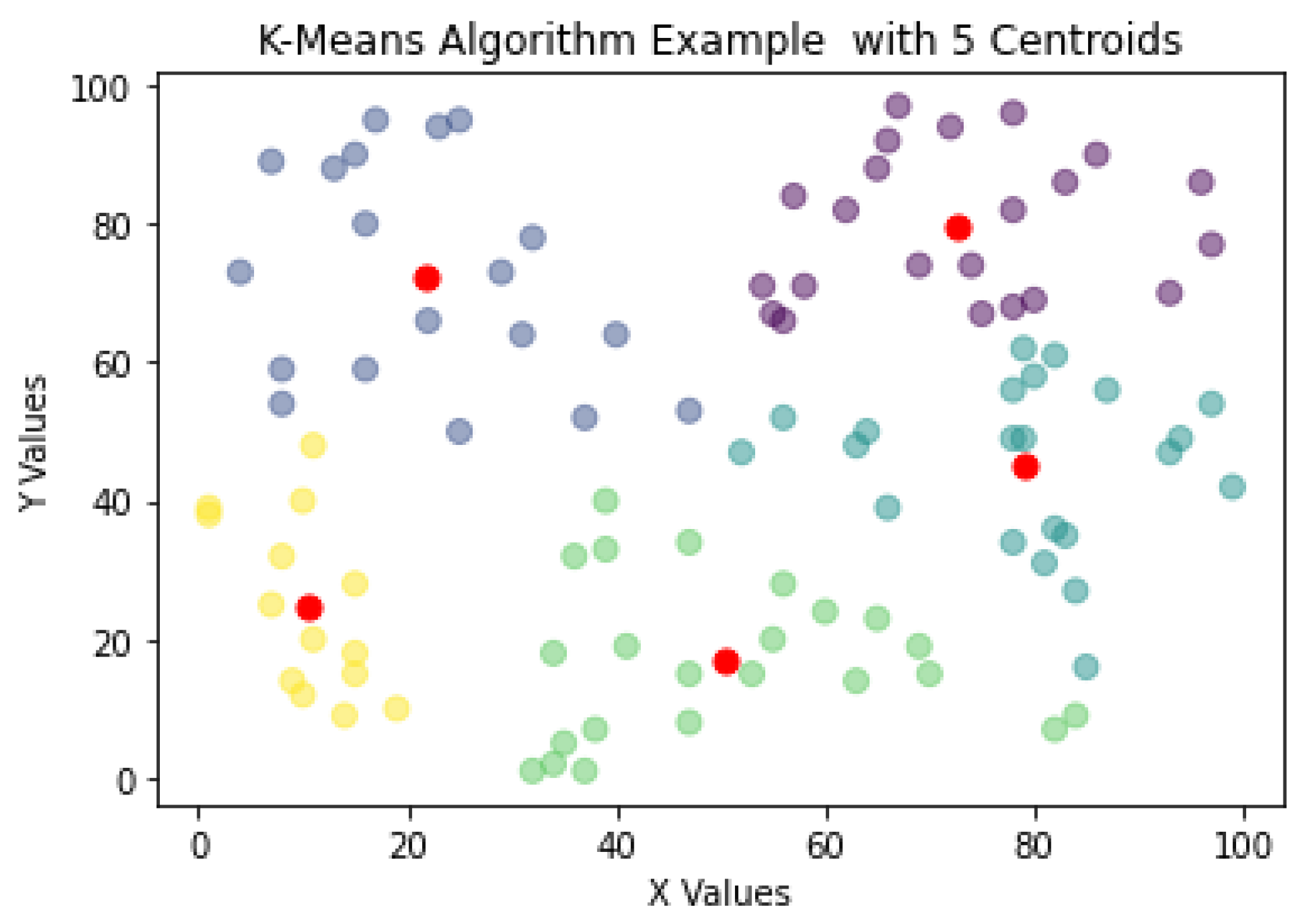
2.3.2. Density-Based Clustering
The Density-Based Clustering (DBC) algorithm is contingent on the idea that datasets contain dense data point regions separated by low regions of data points. In contrast to the K-means algorithm, the DBC algorithms do not need a predetermined k value. Discarding the k value allows for the DBC algorithms to find the number of clusters present in a dataset by analyzing the density distribution of data points in space. An advantage of these algorithms in comparison to the K-means is that it can discern noise and outliers in the data. The noise and outliers are presented as low regions of data point density. In other words, the K-means algorithm would pull these outliers into a cluster due to its k constraint while the DBC would inherently leave them alone. Regarding the use of the DBC algorithms in NDT, many papers predominantly use a branch of the DBC which is the Density-Based Spatial Clustering Applications with Noise (DBSCAN). The DBSCAN leverages a data point’s density reachability and density connectivity [19][16]. The density reachability specifies the maximum distance of two data points to be considered neighbors and part of the same cluster. On the other hand, the density connectivity specifies the minimum number data points needed to define a cluster in a region of space. The fields of Civil and Manufacturing Engineering predominantly use the DBSCAN algorithm to monitor the structural health of materials. The study in [20][17] explores Ultrasonic Testing (UT) to inspect the pressures of tubes in the of the Ontario Hydro. Canada’s system, Channel Inspection and Gauging Apparatus for Reactors (CIGAR) uses UT to obtain volumetric images of the pipelines and assess defective regions in them. The statistical properties of the ultrasonic signals are mapped as data points in space, from which the DBSCAN can conduct its analysis [21][18]. An example of the DBSCAN algorithm in use can be observed in Figure 3. In this case, the algorithm constructed an analysis based on three clusters created by three dense regions encountered in the dataset. Furthermore, in this example the DBSCAN found 18 points of noise in the dataset.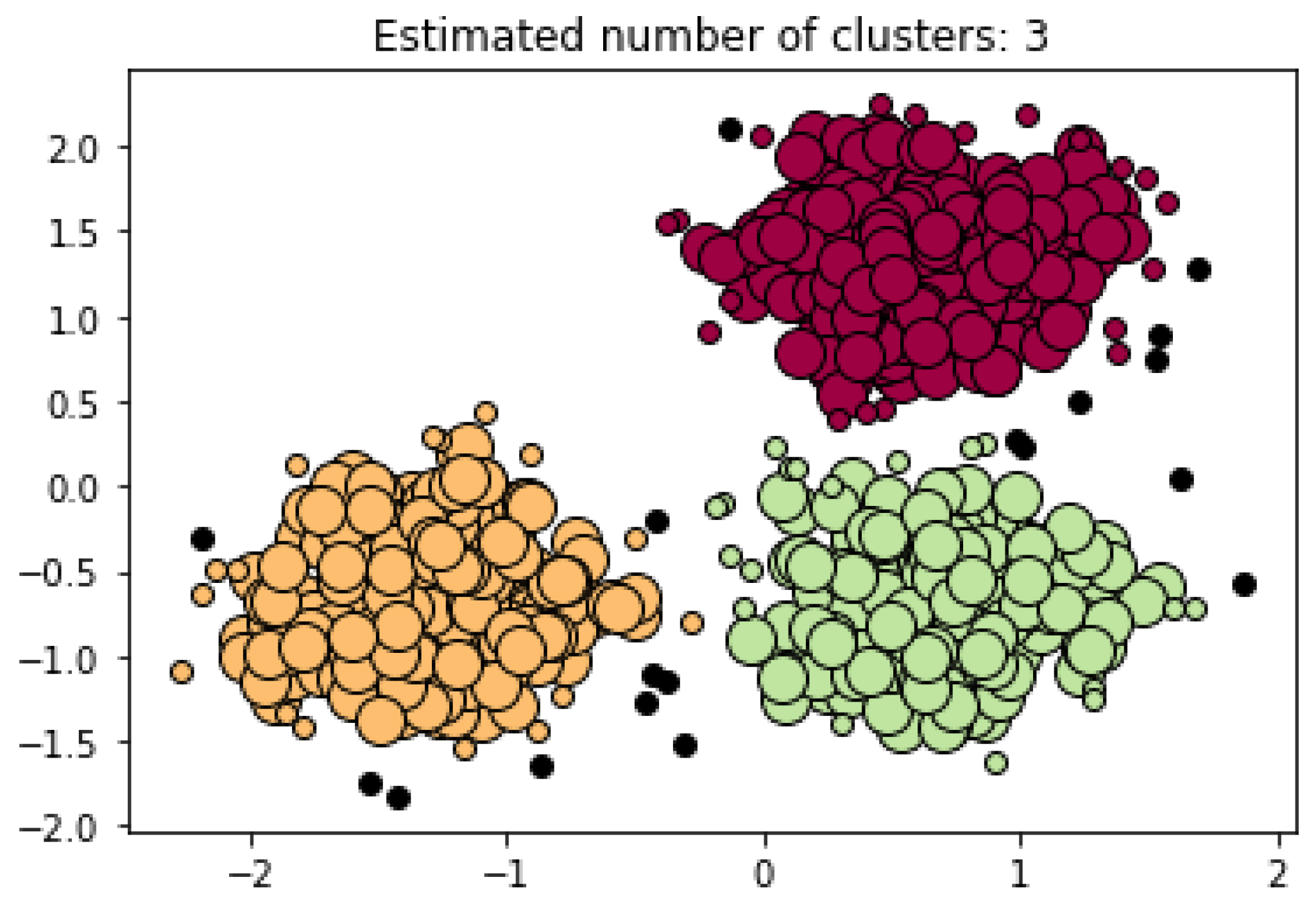
2.3.3. Spectral Clustering
Spectral Clustering is the machine learning method in which the data points in the data set are treated as nodes of a graph. This algorithm is rooted in graph theory and is treated as a graph partitioning problem. The end goal of spectral clustering is to cluster data that is connected but not necessarily in round cluster shapes, as seen in Figure 4. The nodes, or data points, in a data set are projected into a low-dimensional space where connectivity clusters can be achieved. The first step of conducting this algorithm is to compute a similarity graph. The similarity graph is analogous to cluster formation.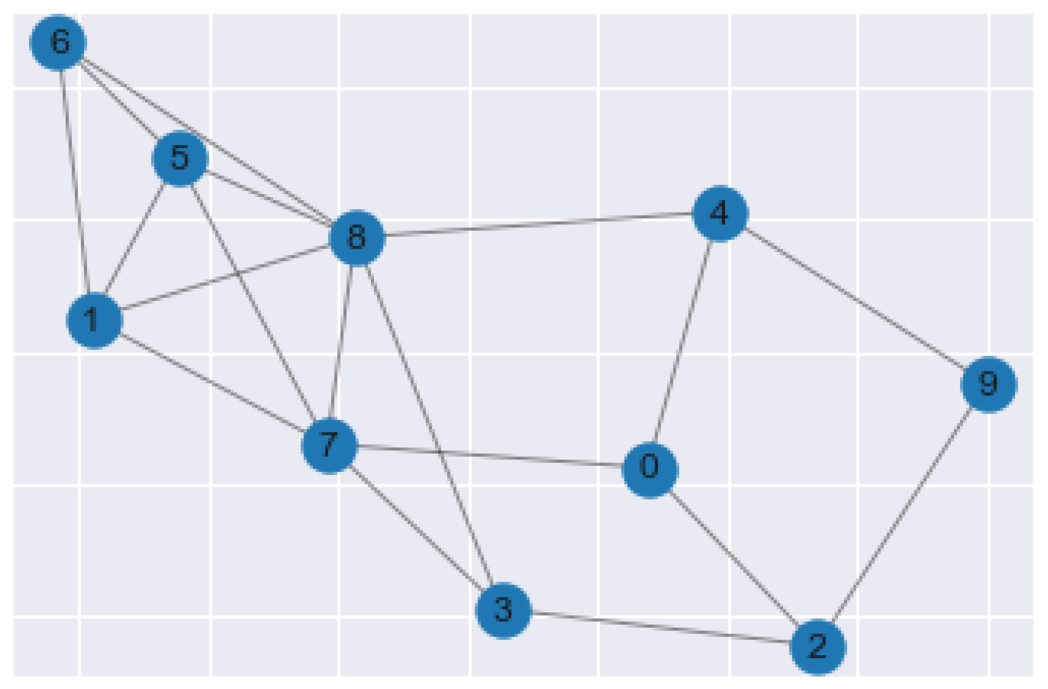
2.3.4. Hierarchical Clustering
Hierarchical clustering is an analytical algorithm used to compute clusters of data points. This type of clustering algorithm is subdivided into two different techniques, agglomerative and divisive. The agglomerative technique imposes that each data point starts as its cluster. Furthermore, the algorithm computes a proximity matrix from each point in space. In every iteration, the algorithm merges the two closest pairs of clusters and a new proximity matrix is computed. There exist four forms of cluster linkage to conduct additive hierarchical clustering. Complete linkage computes the similarity of the furthest pairs in the dataset; however, it is prone to errors if there exist outliers. Single linkage works similarly, but it conducts this comparison between the closest data points. In the same fashion as the previous linkage processes, centroid linkage compares the centroids of each cluster and merges them given found similarities. The last linkage method, group average, finds similarities between the overall clusters and merges them. The linkage process is repeated until a predetermined number of clusters is achieved. The optimal way of describing the additive hierarchical clustering is by creating a dendrogram, as shown in Figure 5.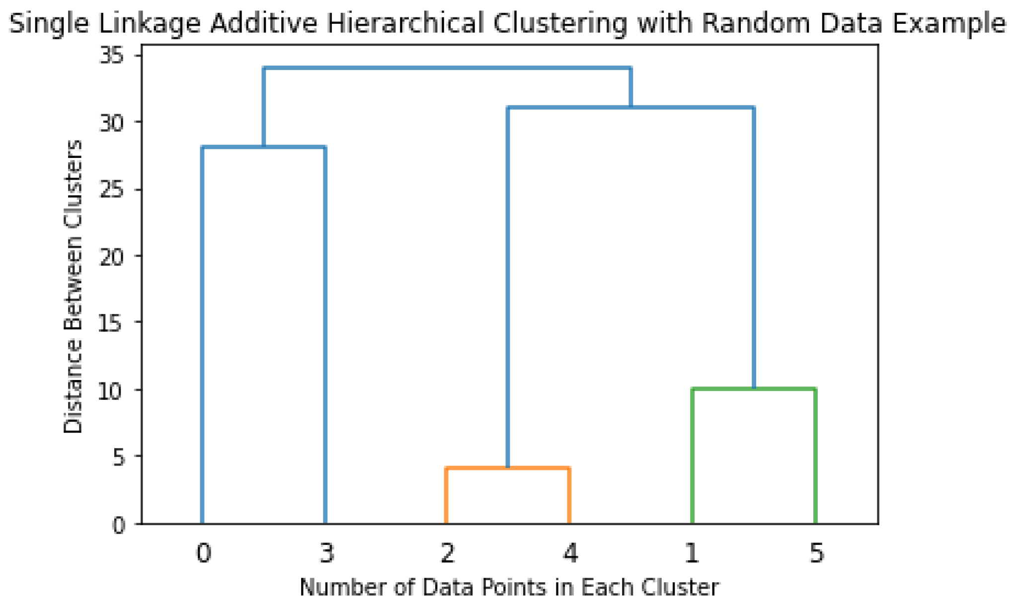
2.4. Association Analysis
2.5. Supervised Learning
Supervised learning is a branch of ML in which the user feeds labeled and classified data to the machine learning algorithms. This data-input methodology helps the algorithm to detect the relationships and patterns faster. Supervised learning is often divided into different categories based on the desired output. The first category in supervised learning is the algorithms with a discrete classification end goal. These algorithms are trained to differentiate among different classification categories from which they were previously trained. The input is analyzed by the supervised learning algorithm and placed in a category that the algorithm finds more suitable given the information extracted from the input (show a feature map and classification examples, very general). The second category of supervised learning is made of algorithms that produce a continuous output (e.g., Regression Analysis) [15].2.5.1. Support Vector Machine
One of the techniques in non-destructive testing that classifies and at the same time obtains a regression from the input data is the Support Vector Machine (SVM) algorithm. This algorithm creates support vector representations from fed labeled examples to properly classify said labels. The support vectors for each class are the most difficult points to classify since they are the closest to the boundary that separates those classes. The separating hyperplanes serve as the plane that separates data into different classes and is highly effective in multidimensional data classification (e.g., two or more classes). One can observe the hyperplane as a line that separates the data in a two-dimensional plane into three different classes, as seen in Figure 6. This line can then be expanded into higher dimensionalities, e.g., a hyperplane, when more classes are introduced in the data.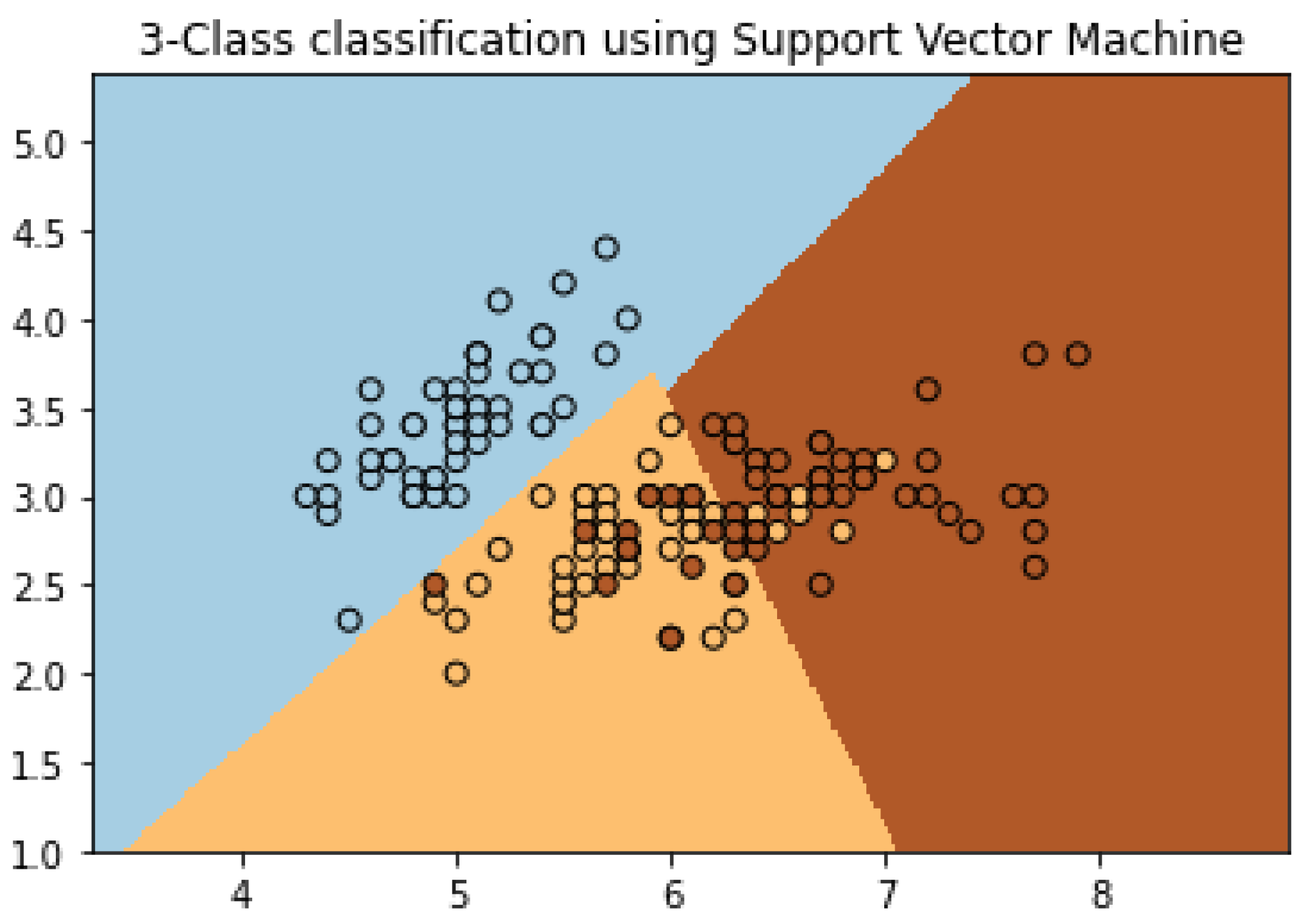
2.5.2. K-Nearest Neighbor
2.5.3. Neural Networks
Neural networks are machine learning algorithms inspired by the workings of the biological neurons of the human brain. This approach is also referred as “deep learning”. These algorithms are built upon stacking node layers made up of an input layer, output layer, and hidden layers. All individual nodes in a node layer have a specific value that activates them. Once a node is activated, it will send information to next node layer. The connections between the nodes are represented by a number, also known as the weight. The weight also holds influence on the nodes, meaning the higher the weight the more leverage it has on the network. In many cases, the neural network has a fully connected design which allows feed forward and feedback information. With this structure, the neural network can deduct information and improve itself based on previous decisions. One of the pillar neural networks in Artificial Intelligence is the LeNet 5 network created by Yann LeCun, et al. [32][21]. This network was developed to recognize handwritten digits and has been a base for many new and emerging networks in the field. Stemming from the same branch as LeNet 5, the famous Convolutional Neural Networks (CNN) have emerged. The widely popular AlexNet [33][22], a CNN variation, has been implemented across several fields to understand nonlinear data for classification. Figure 7 showcases the architectural design of AlexNet.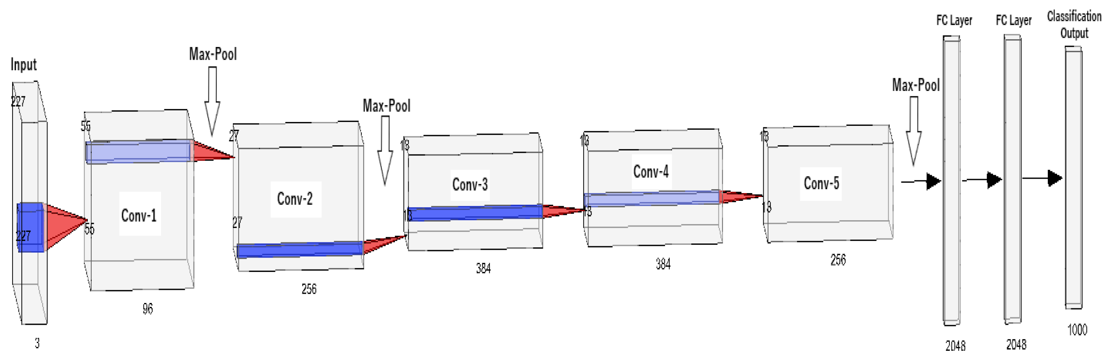
2.6. Feature Extraction
2.7. Machine Vision
References
- Bray, D.E.; Stanley, R.K. Nondestructive Evaluation: A Tool in Design, Manufacturing, and Service; CRC Press: Boca Raton, FL, USA, 2018.
- Koester, L.W.; Bond, L.J.; Taheri, H.; Collins, P.C. Nondestructive evaluation of additively manufactured metallic parts: In situ and post deposition. In Additive Manufacturing for the Aerospace Industry; Elsevier: Amsterdam, The Netherlands, 2019; pp. 401–417.
- Ida, N.; Meyendorf, N. Handbook of Advanced Nondestructive Evaluation; Springer International Publishing: Cham, Switzerland, 2019.
- O’Rorke, P.; Morris, S.; Amirfathi, M.; Bond, W.; Clair, D.S. Machine learning for nondestructive evaluation. In Machine Learning Proceedings 1991; Elsevier: Amsterdam, The Netherlands, 1991; pp. 620–624.
- Ph Papaelias, M.; Roberts, C.; Davis, C.L. A review on non-destructive evaluation of rails: State-of-the-art and future development. Proc. Inst. Mech. Eng. Part F J. Rail Rapid Transit 2008, 222, 367–384.
- Popovics, J.S. Nondestructive evaluation: Past, present, and future. J. Mater. Civ. Eng. 2003, 15, 211.
- Mineo, C.; Herbert, D.; Morozov, M.; Pierce, S.; Nicholson, P.; Cooper, I. Robotic non-destructive inspection. In Proceedings of the 51st Annual Conference of the British Institute of Non-Destructive Testing, Northamptonshire, UK, 11–13 September 2012; pp. 345–352.
- Ahmed, H.; La, H.M.; Gucunski, N. Review of non-destructive civil infrastructure evaluation for bridges: State-of-the-art robotic platforms, sensors and algorithms. Sensors 2020, 20, 3954.
- Gardner, P.; Fuentes, R.; Dervilis, N.; Mineo, C.; Pierce, S.; Cross, E.; Worden, K. Machine learning at the interface of structural health monitoring and non-destructive evaluation. Philos. Trans. R. Soc. A 2020, 378, 20190581.
- Osman, A.; Duan, Y.; Kaftandjian, V. Applied Artificial Intelligence in NDE. In Handbook of Nondestructive Evaluation 4.0; Springer: Berlin/Heidelberg, Germany, 2021; pp. 1–35.
- Wunderlich, C.; Tschöpe, C.; Duckhorn, F. Advanced methods in NDE using machine learning approaches. AIP Conf. Proc. 2018, 1949, 020022.
- Shrifan, N.H.; Akbar, M.F.; Isa, N.A.M. Prospect of using artificial intelligence for microwave nondestructive testing technique: A review. IEEE Access 2019, 7, 110628–110650.
- Siegel, M. Automation for nondestructive inspection of aircraft. In Proceedings of the Conference on Intelligent Robots in Factory, Field, Space, and Service, Houston, TX, USA, 21–24 March 1994; p. 1223.
- Gemander, F. Machine Learning: Basics and NDT Applications. 2019. Available online: https://wiki.tum.de/display/zfp/Machine+Learning%3A+Basics+and+NDT+Applications (accessed on 10 March 2022).
- Harley, J.B.; Sparkman, D. Machine learning and NDE: Past, present, and future. AIP Conf. Proc. 2019, 2102, 090001.
- Ester, M.; Kriegel, H.P.; Sander, J.; Xu, X. A density-based algorithm for discovering clusters in large spatial databases with noise. In Proceedings of the Second International Conference on Knowledge Discovery and Data Mining, Portland, OR, USA, 2–4 August 1996; Volume 96, pp. 226–231.
- Baron, J.; Dolbey, M.; Erven, J.; Booth, D.; Murray, D. Improved pressure tube inspection in Candu reactors. Nucl. Eng. Int. 1981, 26, 45–48.
- Kumar, N.P.; Patankar, V.; Kulkarni, M. Ultrasonic Gauging and Imaging of Metallic Tubes and Pipes: A Review; International Atomic Energy Agency (IAEA): Vienna, Austria, 2020.
- Pedregosa, F.; Varoquaux, G.; Gramfort, A.; Michel, V.; Thirion, B.; Grisel, O.; Blondel, M.; Prettenhofer, P.; Weiss, R.; Dubourg, V.; et al. Scikit-learn: Machine Learning in Python. J. Mach. Learn. Res. 2011, 12, 2825–2830.
- Taheri, H.; Koester, L.W.; Bigelow, T.A.; Faierson, E.J.; Bond, L.J. In situ additive manufacturing process monitoring with an acoustic technique: Clustering performance evaluation using K-means algorithm. J. Manuf. Sci. Eng. 2019, 141, 041011.
- LeCun, Y.; Jackel, L.; Bottou, L.; Brunot, A.; Cortes, C.; Denker, J.; Drucker, H.; Guyon, I.; Muller, U.; Sackinger, E.; et al. Comparison of learning algorithms for handwritten digit recognition. In Proceedings of the International Conference on Artificial Neural Networks, Perth, Australia, 27 November–1 December 1995; Volume 60, pp. 53–60.
- Krizhevsky, A.; Sutskever, I.; Hinton, G.E. Imagenet classification with deep convolutional neural networks. Adv. Neural Inf. Process. Syst. 2012, 25, 1097–1105.
- Radkowski, R.; Garrett, T.; Holland, S.D. 3D machine vision technology for automatic data integration of ultrasonic data. In Proceedings of the QNDE 2019: 46th Annual Review of Progress in Quantitative Nondestructive Evaluation, Portland, OR, USA, 14–18 July 2019.
- Addamani, R.; Ravindra, H.V.; Gayathri Devi, S.; Gonchikar, U. Assessment of Weld Bead Performance for Pulsed Gas Metal Arc Welding (P-GMAW) Using Acoustic Emission (AE) and Machine Vision (MV) Signals Through NDT Methods for SS 304 Material. In ASME International Mechanical Engineering Congress and Exposition; American Society of Mechanical Engineers: New York, NY, USA, 2020; Volume 84485, p. V02AT02A002.
- Johnson, J.T. Defect and Thickness Inspection System for Cast Thin Films Using Machine Vision and Full-Field Transmission Densitometry. Ph.D. Thesis, Georgia Institute of Technology, Atlanta, GA, USA, 2009.
- Ye, X.W.; Dong, C.Z.; Liu, T. A review of machine vision-based structural health monitoring: Methodologies and applications. J. Sensors 2016, 2016, 7103039.
- Tang, Y.; Lin, Y.; Huang, X.; Yao, M.; Huang, Z.; Zou, X. Grand challenges of machine-vision technology in civil structural health monitoring. In Artificial Intelligence Evolution; Universal Wiser Publisher: Singapore, 2020; pp. 8–16.
- Dawood, T.; Zhu, Z.; Zayed, T. Machine vision-based model for spalling detection and quantification in subway networks. Autom. Constr. 2017, 81, 149–160.