Radar Signal Processing Fundamentals

Radar Signal Processing Fundamentals: Comparison

Please note this is a comparison between Version 2 by Sirius Huang and Version 1 by Yi Zhou.

Knowledge of radar signal processing is essential for the development of a deep radar perception system. Different radar devices vary in their sensing capabilities. It is important to leverage radar domain knowledge to understand the performance boundary, find key scenarios, and solve critical problems.

automotive radars
radar signal processing
open-source radar toolbox

1. FMCW Radar Signal Processing

Off-the-shelf automotive radars operate with a sequence of linear frequency-modulated continuous-wave (FMCW) signals to simultaneously measure range, angle, and velocity. According to regulations, automotive radar is allowed to use two frequency bands in millimetre waves: 24 GHz (24–24.25 GHz) and 77 GHz (77–79 GHz). There is a trend towards 77 GHz due to its larger bandwidth (76–77 GHz for long-range and 77–81 GHz for short-range), higher Doppler resolution, and smaller antennas [9]^[1]. As shown in Figure 1, the FMCW signal is characterised by the start frequency (also known as the carrier frequency)

f_{c}

f c , the sweep bandwidth B, the chirp duration

T_{c}

, and the slope

S = B / T_{c}

. During one chirp duration, the frequency increases linearly from

f_{c}

f c to

f c + B

f_{c} + B

with a slope of S. One FMCW waveform is referred to as a chirp, and radar transmits a frame of

N_{c}

chirps equally spaced by chirp cycle time

T_{c}

. The total time

T_{f} = N_{c} T_{c}

is called the frame time, also known as the time on target (TOT). In order to avoid the need for high-speed sampling, a frequency mixer combines the received signal with the transmitted signal to produce two signals with sum frequency

f_{T} (t) + f_{R} (t)

and difference frequency

f_{T} (t) - f_{R} (t)

. Then, a low-pass filter is used to filter out the sum frequency component and obtain the intermediate frequency (IF) signal. In this way, FMCW radar can achieve GHz performance with only MHz sampling. In practice, a quadrature mixer is used to improve the noise figure [10]^[2], resulting in a complex exponential IF signal as

x_{IF} (t) = A e^{j (2 π f_{IF} t + ϕ_{IF})}

where A is the amplitude,

f IF = f T ( t ) − f R ( t )

f_{IF} = f_{T} (t) - f_{R} (t)

is referred to as the beat frequency, and

ϕ_{IF}

is the phase of the IF signal. Next, the IF signal is sampled

N_{s}

times by an ADC converter, resulting in a discrete-time complex signal. Multiple frames of chirp signals are assembled into a two-dimensional matrix. As shown in Figure 1, the dimension of the sampling points within a chirp is referred to as fast time, and the dimension of the chirp index within one frame is referred to as slow time. Assuming one object moving with speed v at distance r, the frequency and phase of the IF signal are given by

f_{IF} = 2 S (r + v T_{c}) c, ϕ_{IF} = 4 π (r + v T_{c}) λ

where

λ = c / f_{c}

is the wavelength of the chirp signal. From (2), we can find that the range and Doppler velocity are coupled. Under the following assumptions: 1. the range variations in slow time caused by target motion can be neglected due to the short frame time; 2. the Doppler frequency in fast time can be neglected compared to the beat frequency by utilising a wideband waveform. Then, range and Doppler can be decoupled. Range can be estimated from the beat frequency as

r = c f_{IF} / 2 S

, and Doppler velocity can be estimated from the phase shift between two chirps as

v = Δ ϕ λ / 4 π T_{c}

. Next, a range DFT is applied in the fast-time dimension to resolve the frequency change, followed by a Doppler DFT in the slow-time dimension to resolve the phase change. As a result, we obtain a 2D complex-valued data matrix called the Range–Doppler (RD) map. In practice, a window function is applied before DFT to reduce sidelobes. The range and the Doppler velocity of a cell in the RD map are given by

r_{k} = k \frac{c}{2 B_{IF}, v_{l} = l \frac{λ}{2 T_{f}}}

where k and l denote the indexes of DFT,

B_{IF}

is the IF bandwidth, and

T_{f}

is the frame time. In practice, FFT is applied due to its computational efficiency. Accordingly, the sequence will be zero-padded to the nearest power of 2 if necessary.

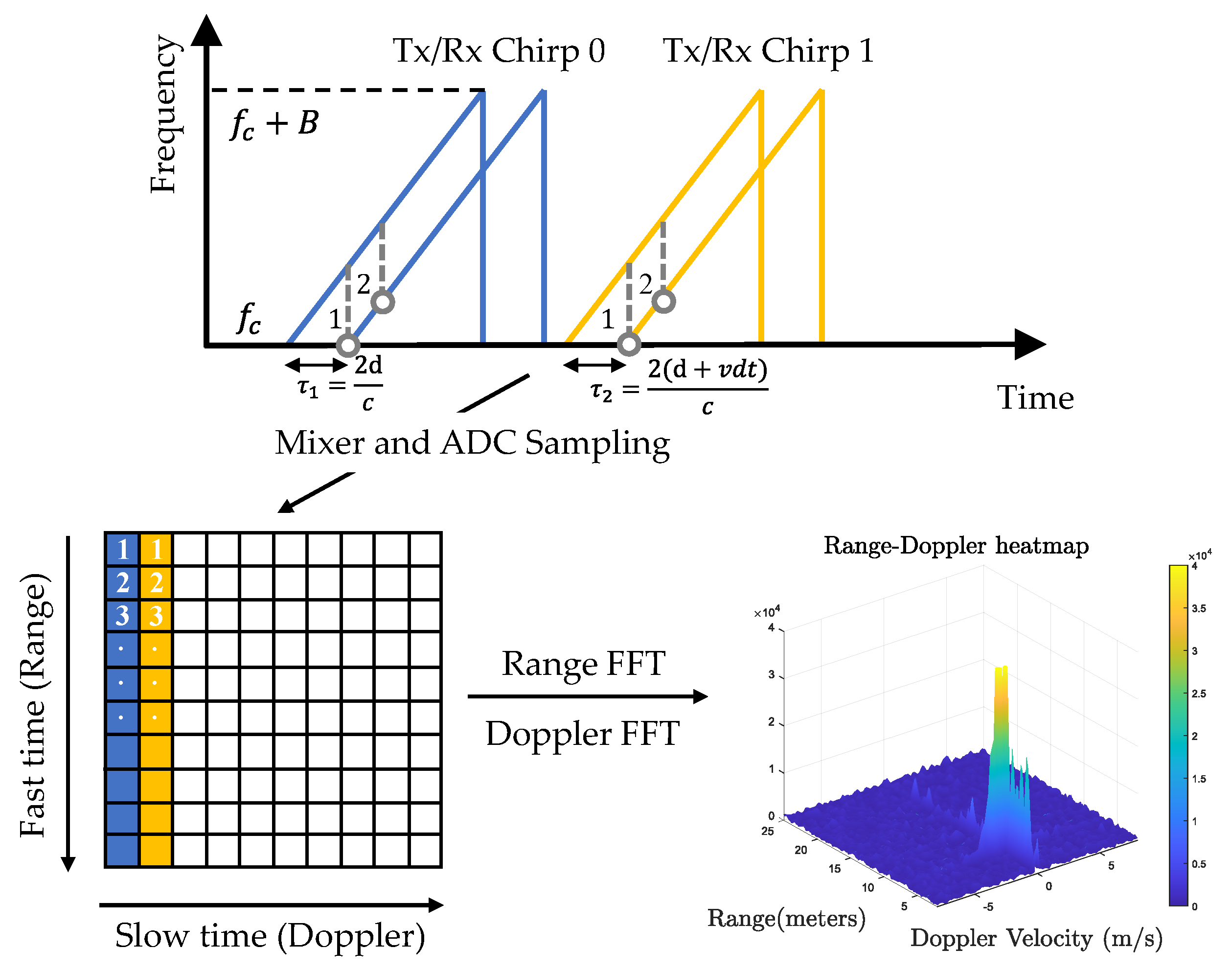
Figure 1. Radar Tx/Rx signals and the resulting range-Doppler map.

Angle information can be obtained using more than one receive or transmit channel. Single-input multiple-output (SIMO) radars utilise a single transmit (Tx) and multiple receive (Rx) antennas for angle estimation. Suppose one object is located in direction

θ

. Similar to Doppler processing, the induced frequency change between two adjacent receive antennas can be neglected, while the induced phase change can be used for calculating the direction of the angle. This phase change is given by

Δ ϕ = 2 π d sin θ / λ

, where d is the inter-antenna spacing. To achieve the maximum unambiguous angle, the spacing can be set to

λ / 2

. Then, a third FFT can be applied to the receive antenna dimension. For conventional radar with a small number of Rx antennas, the sequence is often padded with

N_{FFT} - N_{R x}

zeros to achieve a smooth display of the spectrum. The angle at index

η

is given by

θ_{η} = arcsin η λ N_{FFT}

The angular resolution of a SIMO radar depends on the number of Rx antennas. The maximum number of Rx antennas is limited by the additional cost of signal processing chains on the device [11]^[3]. Multiple-input multiple-output (MIMO) radar operates with multiple channels in both Tx and Rx. As illustrated in Figure 2a, a MIMO radar with

N_{Tx}

Tx antennas and

N_{Rx}

Rx antennas can synthesise a virtual array with

N_{Tx} N_{Rx}

channels. In order to separate the transmit signals at the receiver side, the signals from different Tx antennas should be orthogonal. There are multiple ways to realise waveform orthogonality, such as time-division multiplexing (TDM), frequency-division multiplexing (FDM), and Doppler-division multiplexing (DDM) [12,13]^[4][5]. TDM is widely used for its simplicity. In this mode, different Tx antennas transmit chirp signals in turns, as shown in Figure 2b. Therefore, at the receiver side, different Tx waveforms can be easily separated in the time domain. An additional phase shift compensation [14]^[6] is required to compensate for the motion of detections during the Tx switching time. Another shortcoming of TDM is the reduced detection range due to the loss of transmitting power. DDM is also supported by many radar devices. As shown in Figure 2c, DDM transmits all Tx waveforms simultaneously and separates them in the Doppler domain. In order to realise waveform orthogonality, for the k-th transmitter, a Doppler shift is added to adjacent chirps as

ω_{k} = 2 π (k - 1) N

where N is usually selected as the number of Tx antennas

N_{Tx}

. One drawback of DDM is that its unambiguous Doppler velocity is reduced to

\frac{1}{N}

of the original one. Empty-band DDM [15]^[7] can achieve more robust velocity disambiguation by introducing several empty Doppler sub-bands. Some example codes are provided in the RADIal dataset [16]^[8]. After decoupling the received signals, we can obtain a 3D tensor by stacking RD maps with respect to Tx–Rx pairs. Then, the DOA can be estimated through the angle FFT along the virtual receiver dimension. Some super-resolution methods [17]^[9], such as Capon, MUSIC, and ESPRIT, can be applied to improve angular resolution. The resulting 3D tensor is referred to as the range–azimuth–Doppler (RAD) tensor or radar tensor.

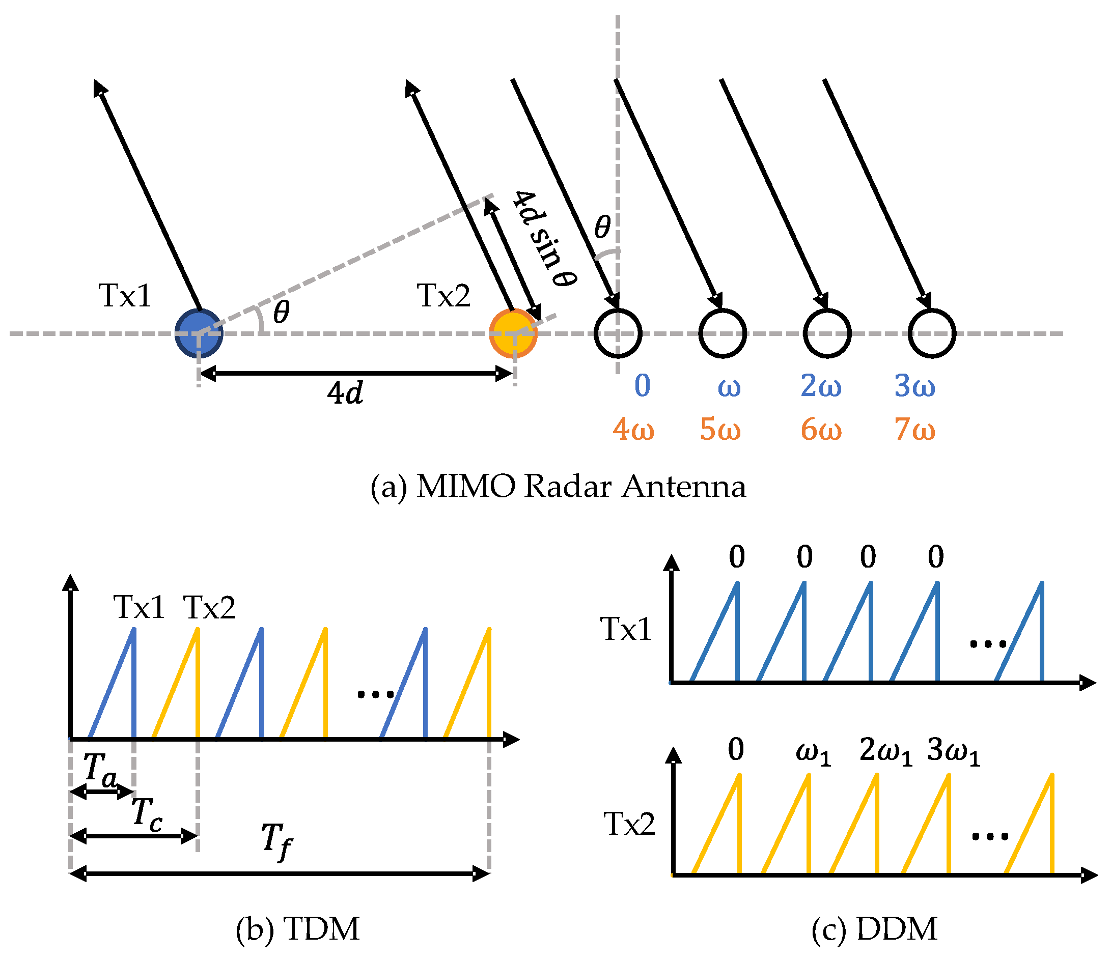
Figure 2. MIMO radar principles. (a) Virtual array configuration of a 2Tx4Rx MIMO radar (b) In TDM mode, Tx1 and Tx2 transmit signals in turns. (c) In DDM mode, a Doppler shift is added to Tx2.

In the radar detection pipeline, RD maps are integrated coherently along the virtual receiver dimension to increase the SNR. Then, a constant false alarm rate (CFAR) detector [18]^[10] is applied to detect peaks in the RD map. Finally, the DOA estimation method is applied for angle estimation. The output is a point cloud with measurements of range, Doppler, and angle. For conventional radars, only the azimuth angle is resolved, while 4D radars output both azimuth and elevation angles. Since radar is usually used in safety-critical applications, a lower CFAR threshold (≤10 dB) is set to achieve high recall. The accuracy of detection is affected by road clutter, interferences, and multi-path effects in complex environments. Therefore, additional spatial–temporal filtering is required to improve accuracy. DBSCAN [19]^[11] is used to cluster radar detections into object-level targets. Clusters with few detections are considered as outliers and, thus, be removed. Further, temporal filtering, such as Kalman filtering, is used to filter out outliers and interpolate missed detections.

2. Radar Performances

The performance of automotive radar can be evaluated in terms of maximum range, maximum Doppler velocity, and field of view (FoV). Equations for these attributes are summarised in Table 1. According to the radar equation, the theoretical maximum detection range is given by

R_{max} = P_{t} G^{2} λ^{2} σ (4 π) 3 P_{min} \sqrt[4]{}

where

P_{t}

is the transmit power,

P_{\min}

is the minimum detectable signal or receiver sensitivity,

λ

is the transmit wavelength,

σ

is the target RCS, and G is the antenna gain. The wavelength is 3.9 mm for automotive 77 GHz radar. The target RCS is a measure of the ability to reflect radar signals back to the radar receiver. It is a statistical quantity that varies with the viewing angle and the target material. According to the test results [20]^[12], smaller objects, such as pedestrians and bikes, have an average RCS value of around 2–3 dBsm, whereas normal vehicles have an average RCS value of around 10 dBsm and large vehicles of around 20 dBsm. The other parameters, such as transmit power, minimum detectable signal, and antenna gain are design parameters aimed at meeting product requirements, as well as regulations. Some typical values for these parameters are summarised in Table 2. In practice, the maximum range is limited by the supported IF bandwidth

B_{IF}

and ADC sampling frequency. The maximum unambiguous velocity is inversely proportional to the chirp duration

T_{c}

. For MIMO radar, the maximum unambiguous angle is dependent on the spacing of antennas d. The theoretical maximum FoV is 180° if

d = λ / 2

. In practice, the FoV is determined by the antenna gain pattern. Another important characteristic is resolution, i.e., the ability to separate two close targets with respect to range, velocity, and angle. As shown in Table 1, high-range resolution requires a large sweep bandwidth B. High Doppler resolution requires a long integration time, i.e., the frame time

N_{c} T_{c}

. The angular resolution depends on the number of virtual receivers

N_{R}

, the object angle

θ

, and the inter-antenna spacing d. For the case of

d = λ / 2

and

θ = 0

°, angular resolution is in a simple form of

2 / N_{R}

. From the perspective of antenna theory, angular resolution can also be featured by the half-power beamwidth, i.e., the 3-dB beamwidth [13]^[5], which is a function of the array aperture D.

Table 1.

Equations for radar performance.

Definition	Equation
Max Unambiguous Range	$R_{m} = \frac{c B_{IF}}{2 S}$
Max Unambiguous Velocity	$v_{m} = \frac{λ}{4 T_{c}}$
Max Unambiguous Angle	$θ_{FoV} = \pm arcsin (\frac{λ}{2 d})$
Range Resolution	$Δ R = \frac{c}{2 B}$

The meaning of parameters is consistent in this section. Refer to Table A1 (in Appendix A) for a quick check of the meaning.

Table 2. Typical automotive radar parameters [17].

Typical automotive radar parameters ^[9].

Parameter	Range
Transit power (dBm)	10–13
TX/RX antenna gain (dBi)	10–25
Receiver noise figure (dB)	10–20
Velocity Resolution
Target RCS (dBsm)	(−10)–20	$Δ v = \frac{λ}{2 N_{c} T_{c}}$
Angular Resolution
Receiver sensitivity (dBm)	(−120)–(−115)	$Δ θ_{res} = \frac{λ}{N_{R} d c o s (θ)}$
Minimum SNR (dB)	$Δ θ_{res} = \frac{λ}{N_{R} d c o s (θ)}$
10–20	3 dB Beamwidth	$Δ θ_{3 dB} = 2 arcsin \frac{1.4 λ}{π D}$

In practice, different types of automotive radar are designed for different scenarios. Long-range radar (LRR) achieves a long detection range and a high angular resolution at the cost of a smaller FoV. Short-range radar (SRR) uses MIMO techniques to achieve a high angular resolution and large FoV. In addition, different chirp configurations [21]^[13] are used for different applications. For example, long-range radar needs to detect fast-moving vehicles at distances and, therefore, utilises a small ramp slope for long-distance detection, a long chirp integration time to increase the SNR, a small chirp duration to increase the maximum velocity, and a short chirp duration for high-velocity resolution [22]^[14]. Short-range radar needs to detect vulnerable road users (VRUs) close to the vehicle and, therefore, utilises a higher sweep bandwidth for high-range resolution at the cost of a short range. Multi-mode radar [21]^[13] can work in different modes simultaneously by sending chirps that are switched sequentially with different configurations.

3. Open-Source Radar Toolbox

Commercial off-the-shelf radar products can only output point clouds. They can be configured to output either raw point clouds, sometimes referred to as radar detections, or clustered objects with tracked IDs. The signal processing algorithm inside it is a black box and cannot be modified. Alternatively, TI mm-wave radars have been widely used in academic research because of their public nature and flexibility. They support configurable chirps [21]^[13] and different MIMO modes [11]^[3] to adapt to different tasks. TI also provides a mmWave studio, which provides GUIs for radar setup, data capturing, signal processing, and visualisation. In addition, there are some open-source radar signal processing toolboxes for TI devices, for example RaDICaL SDK [23^[15][16],24], PyRapid [25]^[17], OpenRadar [26]^[18], and Pymmw [27]^[19]. These toolboxes enable researchers to build their own datasets using TI devices. While there is a growing number of public radar datasets, most of them provide limited information about the radar configurations they use. This makes it difficult to make a fair comparison between algorithms trained on different datasets. The open radar initiative [28]^[20] provides a guideline for radar configuration and encourages researchers to expand this dataset by using the radar device with the same configuration.

Appendix A

Table A1.

Parameters used in the radar signal processing section.

Parameter	Meaning	Parameter	Meaning
c	Light Speed (m/s	$^{2}$	)	$N_{T x}$	Number of Tx Antennas
$λ$	Wavelength (m)	$N_{R x}$	Number of Rx Antennas
$f_{c}$	Carrier Frequency (Hz)	d	Inter Antenna Spacing (m)
B	Sweep Bandwidth (dB)	D	Array Aperture (m)
S	Chirp Slope	$P_{t}$	Transmit Power (dBW)
$N_{c}$	Number of Chirps	G	Antenna Gain (dB)
$T_{c}$	Chirp Duration (s)	$P_{m i n}$	Minimum Detectable Power (dBw)
$T_{f}$	Frame Duration (s)	$σ$	Radar Cross-Section (dBm	$^{2}$	)
$B_{I F}$	IF Bandwidth (dB)	$S N R$	Signal-to-Noise Ratio

References

Hakobyan, G.; Yang, B. High-performance automotive radar: A review of signal processing algorithms and modulation schemes. IEEE Signal Process. Mag. 2019, 36, 32–44.
Ramasubramanian, K.; Instruments, T. Using a Complex-Baseband Architecture in FMCW Radar Systems; Texas Instruments: Dallas, TX, USA, 2017.
Rao, S. MIMO Radar; Application Report SWRA554A; Texas Instruments: Dallas, TX, USA, 2017.
Sun, H.; Brigui, F.; Lesturgie, M. Analysis and comparison of MIMO radar waveforms. In Proceedings of the 2014 International Radar Conference, Lille, France, 13–17 October 2014; pp. 1–6.
Sun, S.; Petropulu, A.P.; Poor, H.V. MIMO radar for advanced driver-assistance systems and autonomous driving: Advantages and challenges. IEEE Signal Process. Mag. 2020, 37, 98–117.
Bechter, J.; Roos, F.; Waldschmidt, C. Compensation of motion-induced phase errors in TDM MIMO radars. IEEE Microw. Wirel. Compon. Lett. 2017, 27, 1164–1166.
Gupta, J. High-End Corner Radar Reference Design. In Design Guide TIDEP-01027; Texas Instruments: Dallas, TX, USA, 2022.
Rebut, J.; Ouaknine, A.; Malik, W.; Pérez, P. RADIal Dataset. 2022. Available online: https://github.com/valeoai/RADIal (accessed on 1 May 2022).
Gamba, J. Radar Signal Processing for Autonomous Driving; Springer: Berlin/Heidelberg, Germany, 2020.
Richards, M.A. Fundamentals of Radar Signal Processing; Tata McGraw-Hill Education: New York, NY, USA, 2005.
Schubert, E.; Sander, J.; Ester, M.; Kriegel, H.P.; Xu, X. DBSCAN revisited, revisited: Why and how you should (still) use DBSCAN. ACM Trans. Database Syst. (TODS) 2017, 42, 1–21.
Muckenhuber, S.; Museljic, E.; Stettinger, G. Performance evaluation of a state-of-the-art automotive radar and corresponding modelling approaches based on a large labeled dataset. J. Intell. Transp. Syst. 2021, 1–20.
Dham, V. Programming chirp parameters in TI radar devices. In Application Report SWRA553; Texas Instruments: Dallas, TX, USA, 2017.
Hasch, J.; Topak, E.; Schnabel, R.; Zwick, T.; Weigel, R.; Waldschmidt, C. Millimeter-wave technology for automotive radar sensors in the 77 GHz frequency band. IEEE Trans. Microw. Theory Tech. 2012, 60, 845–860.
Lim, T.Y.; Markowitz, S.; Do, M.N. RaDICaL Dataset SDK. 2021. Available online: https://github.com/moodoki/radical_sdk (accessed on 1 May 2022).
Lim, T.Y.; Markowitz, S.; Do, M.N. IWR Raw ROS Node. 2021. Available online: https://github.com/moodoki/iwr_raw_rosnode (accessed on 1 May 2022).
Mostafa, A. pyRAPID. 2020. Available online: http://radar.alizadeh.ca (accessed on 1 May 2022).
Pan, E.; Tang, J.; Kosaka, D.; Yao, R.; Gupta, A. OpenRadar. 2019. Available online: https://github.com/presenseradar/openradar (accessed on 1 May 2022).
Constapel, M.; Cimdins, M.; Hellbrück, H. A Practical Toolbox for Getting Started with mmWave FMCW Radar Sensors. In Proceedings of the 4th KuVS/GI Expert Talk on Localization, Lübeck, Germany, 11–12 July 2019.
Gusland, D.; Christiansen, J.M.; Torvik, B.; Fioranelli, F.; Gurbuz, S.Z.; Ritchie, M. Open Radar Initiative: Large Scale Dataset for Benchmarking of micro-Doppler Recognition Algorithms. In Proceedings of the 2021 IEEE Radar Conference (RadarConf21), Atlanta, GA, USA, 7–14 May 2021; pp. 1–6.