Your browser does not fully support modern features. Please upgrade for a smoother experience.
Please note this is a comparison between Version 2 by Conner Chen and Version 1 by Weimin Chen.
Computer vision-based structural deformation monitoring techniques were studied in a large number of applications in the field of structural health monitoring (SHM). Numerous laboratory tests and short-term field applications contributed to the formation of the basic framework of computer vision deformation monitoring systems towards developing long-term stable monitoring in field environments.
- computer vision
- structural deformation monitoring
- field environment
1. Introduction
Transportation infrastructure systems such as bridges, tunnels and railroads are important component systems for national social production and national development. With the tremendous development of social productivity, these transportation infrastructures are tested in two major ways. On the one hand, the tonnage and number of existing means of transportation may exceed the design load-carrying capacity; on the other hand, civil engineering structures including bridges, are subjected to various external loads or disasters (such as fire and earthquakes) during their service life, which in turn reduces the service life of the structures. By carrying out inspection, monitoring, evaluation, and maintenance of these structures, we can ensure the long life and safe service of national infrastructure and transportation arteries, which is of great strategic importance to support the sustainable development of the national economy.
In the past two decades, structural health monitoring (SHM) has emerged with the fundamental purpose of collecting the dynamic response of structures using sensors and then reporting the results to evaluate the structures’ performance. Their wide deployment in realistic engineering structures is limited by the requirement of cumbersome and expensive installation and maintenance of sensor networks and data acquisition systems [1,2,3][1][2][3]. At present, the sensors used for SHM are mainly divided into contact type (linear variable differential transformers (LVDT), optical fiber sensors [4[4][5][6][7][8][9],5,6,7,8,9], accelerometers [10[10][11],11], strain gauges, etc.) and non-contact types (such as global positioning systems (GPS) [12[12][13][14],13,14], laser bibrometers [15], Total Station [16], interferometric radar systems [17], and level computer vision-based sensors). Amongst the existing non-contact sensors, the GPS sensor is easy to install, but the measurement accuracy is limited, usually between 5 mm and 10 mm, and the sampling frequency is limited (i.e., less than 20 Hz) [18,19,20,21,22][18][19][20][21][22]. Xu et al. [23] made a statistical analysis of the data collected using accelerometers and pointed out that the introduction of maximum likelihood estimation in the process of fusion of GPS displacement data and the corresponding acceleration data can improve the accuracy of displacement readings. The accuracy of the laser vibrometer is usually very good, ranging from 0.1 mm to 0.2 mm, but the equipment is expensive and its range is usually less than 30 m [24]. Remote measurements can be performed with better than 0.2 mm accuracy using a total station or level, but the dynamic response of the structure cannot be collected [25,26][25][26].
With the development of computer technology, optical sensors and image processing algorithms, computer vision has been gradually applied in various fields of civil engineering. High-performance cameras are used to collect field images, then various algorithms are used to perform image analysis on a computer to obtain information such as strain, displacement, and inclination. After further processing of these data, the dynamic characteristics such as mode shape, frequency, acceleration and damping ratio can be obtained. Some researchers extract the influence line [27,28][27][28] and the influence surface [29] of a bridge structure from the spatial and temporal distribution information of vehicle loads, which are used as indicators to evaluate the safety performance of the structure. However, the long-term application of computer vision in the field is limited in many ways; for example, the selection of targets, measurement efficiency and accuracy, environment impact (especially the impact of temperature and illuminate changes).
2. System Composition
A computer vision-based structural deformation monitoring system includes an image acquisition system and an image processing system. The image acquisition system includes a camera, lens, and target to collect video images, while the image processing system performs camera calibration, feature extraction, target tracking, and deformation calculation, which purpose is to process the acquired image and calculate the structural deformation. This section will briefly introduce the basic components of the image acquisition system in the computer vision monitoring system. The image processing system will be introduced in Section 3.2.1. Camera
The camera is an important part of the image acquisition system, and its most essential function is to transform received light into an electrical signal through a photosensitive chip and transmit it to the computer. Photosensitive chips can be divided into CCD and CMOS according to the different ways of digital signal transmission. The main differences between them are that CCD has advantages over CMOS in imaging quality, but its cost is much higher than that of CCD, so it is suitable for high-quality image acquisition; CMOS is highly integrated and saves electricity compared with CCD, but the interference of light, electricity and magnetism is serious and its anti-noise ability is weak, so it is more suitable for high-frequency vibration acquisition [30,31][30][31]. The selection of the camera needs to consider the following points: (1) the appropriate chip type and size is to be selected according to the measurement accuracy and application scenario; (2) because of the limited bandwidth, the frame rate and resolution of the camera are contradictory, so the frame rate and resolution should be balanced in camera selection; (3) industrial cameras appear to be the only option for long-term on-site monitoring.2.2. Lens
The lens plays an important role in a computer vision system, and its function is similar to that of the lens in a human eye. It gathers light and directs it ontp the camera sensor to achieve photoelectric conversion. Lenses are divided into fixed-focus lenses [32,33][32][33] and zoom lenses [34]. Fixed-focus lenses are generally used in laboratories, and high-power zoom lens are generally used for long-distance monitoring such as of long-span bridge structures and high-rise buildings. The depth of field is related to the focal length of the lens; the longer the focal length, the shallower the depth of field. The following points need to be considered in the selection of shots: (1) a low distortion lens can improve the calibration efficiency; (2) an appropriate focal length for the camera sensor size, camera resolution and measuring distance should be selected; (3) a high-power zoom lens is appropriate for medium and long-distance shooting.2.3. Target
The selection of targets directly affects the measurement accuracy, and an appropriate target can be selected according to the required accuracy. There are mainly two kinds of target: artificial targets and natural targets. Ye et al. [35] introduced six types of artificial targets [19,36,37][19][36][37] (flat panels with regular or irregular patterns, artificial light sources, irregular artificial speckles, regular boundaries of artificial speckle bands, and laser spots) and a class of natural targets [38,39][38][39]. Artificial targets can provide high accuracy and are robust to changes in the external environment, just as artificial light sources can improve the robustness of targets in light and the possibility of monitoring at night. The disadvantage of artificial target is that they need to be installed manually, which may change the dynamic characteristics of the structure. Natural targets rely on the surface texture or geometric shape of the structure, which is sensitive to changes of the external environment, and their accuracy is not high. The following points should be noted in the selection of targets: (1) when the target installation conditions permit, priority should be given to selecting artificial targets to obtain stable measurement results; (2) the selection of targets should correspond to the target tracking algorithm in order to achieve better monitoring results.3. Basic Process
The flowchart of deformation monitoring based on computer vision is shown in Figure 1, and can be summarized as follows: (1) assemble the camera and lens to aim at artificial or natural targets, and then acquire images; (2) calibrate the camera; (3) extract features or templates from the first frame of the image, then track these features again in other image frames; (4) calculate the deformation. The following is a brief description of camera calibration, feature extraction, target tracking and deformation calculation.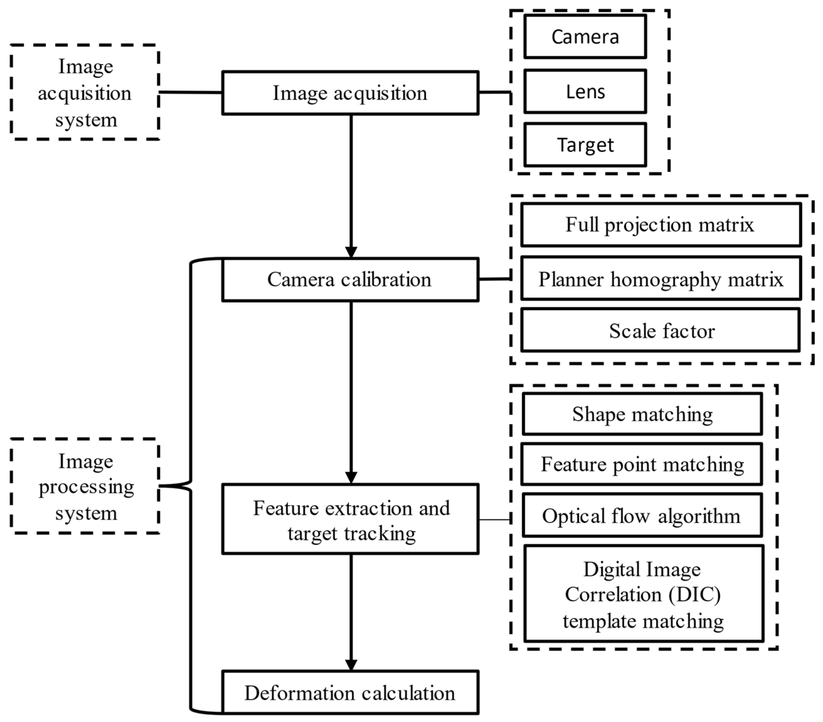
Figure 1.
Process of deformation monitoring based on computer vision.
3.1. Image Acquisition
Image acquisition includes these steps: (1) determine the position to be monitored; (2) arrange artificial targets or use natural targets on the measurement points; (3) select an appropriate camera and lens; (4) assemble the camera lens and set it firmly on a relatively stationary object; (5) aim at the target and acquire images.3.2. Camera Calibration
Camera calibration [40] is the process of determining a set of camera parameters which associate real points with points in the image. Camera parameters can be divided into internal parameters and external parameters: internal parameters define the geometric and optical characteristics of the camera, while external parameters describe the rotation and translation of the image coordinate system relative to a predefined global coordinate system [41]. In order to obtain the structural displacement from the captured video image, it is necessary to establish the transformation relationship from physical coordinates to pixel coordinates. The common coordinate conversion methods are full projection matrix, planar homography matrix, and scale factor.3.2.1. Full Projection Matrix
The full projection matrix transformation reflects the whole projection transformation process from 3D object to 2D image plane. The camera internal matrix and external matrix can be obtained by observing a calibration board, which can be used to eliminate image distortion and has a high accuracy [42]. Commonly used calibration boards include checkerboard [43] and dot lattice [44]. Figure 2a shows the relationship between the camera coordinate system, the image coordinate system and the world coordinate system. A point T (X, Y, Z) in the real 3D world appears at the position t (x, y) in the image coordinate system after the projection transformation (where the origin of the coordinates is P). The relationship between the pixel coordinate system and the image coordinate system is shown in Figure 2b. Therefore, the equation for converting a point from a coordinate in the 3D world coordinate system to a coordinate in the pixel coordinate system is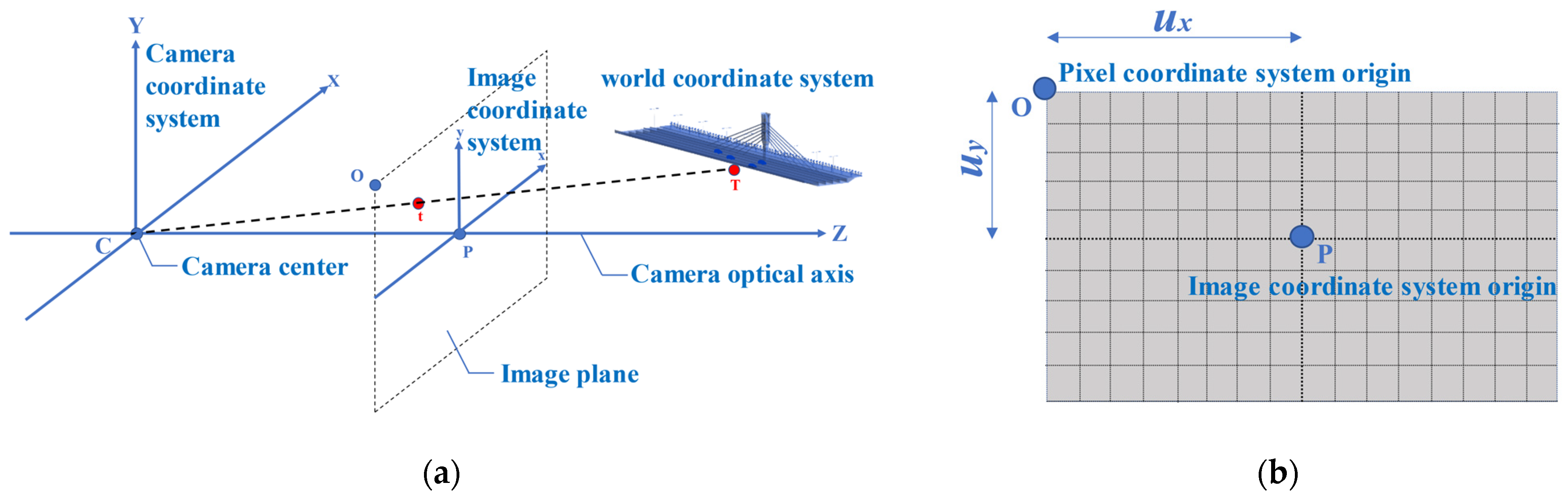
Figure 2. (a) Relationship among the camera coordinate system, the image coordinate system, and the world coordinate system; and (b) Relationship between the pixel coordinate system and the image coordinate system.
3.2.2. Planar Homography Matrix
In practical engineering applications, the above calibration process is relatively complex. To simplify the process, Equation (1) can be expressed3.2.3. Scale Factor
The scale factor (S) provides a simple and practical calibration method. As shown in Figure 3a, when the camera optical axis is perpendicular to the surface of the object, S (unit: mm/pixel) can be obtained based on the internal parameters of the camera (focal length, pixel size) and the external parameters of the camera and the surface of the object (measurement distance) in a simplified calculationfrom the simplified formula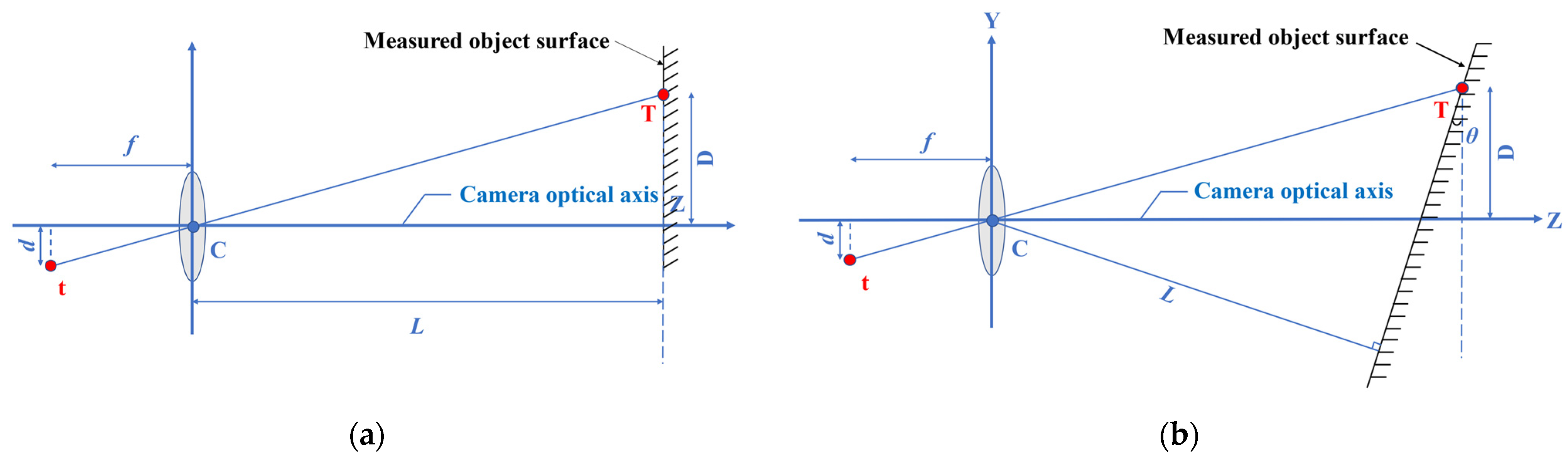
Figure 3. Scaling factor calibration method. (a) Camera optical axis orthogonal to measured object surface; (b) Camera optical axis intersecting obliquely with measured object surface.
3.3. Feature Extraction and Target Tracking
Feature extraction is used to obtain the unique information in the image (such as shape features, feature points, grayscale features, and particle features). The purpose of target tracking algorithms is to find these features again in other image frames. Common target tracking algorithms in civil engineering structural deformation monitoring include shape matching, feature point matching, optical flow estimation and digital image correlation (DIC) template matching.3.3.1. Shape Matching
In an image, shape is a description of an edge or region, and shape matching is an image matching algorithm to identify and locate measured objects through image edge features. There are many algorithms for edge detection, such as Zernike operator [56], Roberts operator, Sobel operator [57], Log operator [58], Canny operator [59] and generalized Hough algorithm [60]. Among them, the Canny operator is widely used because of its high performance [61,62][61][62]. The principle of shape matching is relatively simple and can be used for displacement monitoring of structures with obvious shapes. The advantages are: (1) the calculation is relatively simple and the matching speed is fast; (2) it is robust to change of illumination because it tracks the geometric boundary of the object; (3) this measurement has an advantage for linear structures such as slings.3.3.2. Feature Point Matching
Feature point matching is a target tracking method based on feature extraction and matching. The key points in computer vision are those which are stable, unique and invariant to image transformation, such as building corners, connection bolts, or other shaped targets [63,64][63][64]. The common methods of feature point detection include Harris Corner [65], Shi–Tomasi Corner [66], scale invariant feature transform (SIFT) [32[32][67],67], speed-up robust feature (SURF) [68], binary robust independent elementary features (BRIEF) [69], binary robust invariant scalable keypoint (BRISK) [70], and fast retina keypoint (FREAK) [71]. A feature point matching algorithm needs to select appropriate feature descriptors according to the measurement object to describe feature points mathematically and carry out image registration. It is usually suitable for structures with rich textures or certain shapes (Such as circle, hexagon or rectangle). Feature point matching has the following characteristics: (1) it deals with the whole image area and has accurate matching performance [72]; (2) it extracts texture features of the structure and is not sensitive to illumination and shape transformation; (3) the greater the number of feature points used, the higher is the precision (however, this increases the calculation time).3.3.3. Optical Flow Algorithm
Optical flow algorithm is an image registration technique in which the surface motion in a three-dimensional environment is approximated as a two-dimensional field by using the spatio-temporal pattern of image intensity [73]. The optical flow algorithm can accurately provide the velocity and displacement of the object by tracking the trajectories of pixels, but it has great limitations and makes the following assumptions [74]: (1) the brightness of objects in adjacent frames remains unchanged; (2) the motion of objects in adjacent frames is small enough; (3) the motion between adjacent pixels is consistent [75]. Common optical flow algorithms include Lucas–Kanade [76,77][76][77], Horn–Schunck method [78], Farneback method [79], block match method [80], and phase-based optical flow [45,81,82][45][81][82]. Among those, Lucas–Kanade is fast and easy to implement, and it can perform motion tracking in the selected measurement area, especially of robust feature points, while other algorithms need to calculate every pixel in the image, which is slow. The optical flow algorithm is similar to the feature point matching algorithm in that it tracks feature points on the image and prefers target patterns with distinct and robust features over the whole test period. The optical flow algorithm has the following characteristics: (1) target features need to be clear; (2) sensitivity to illumination changes; (3) only motion components perpendicular to local edge direction can be detected, such as bridge cable vibration; (4) optical flow describes the motion information of the image brightness and is more suitable for measuring dynamic displacement.3.3.4. DIC Template Matching
The basic principle of DIC is to compare the same points (or pixels) recorded between two images before and after deformation, and to calculate the motion of each point [83]. As a representative non-interference optical technique, DIC has the advantage of continuous measurement of the whole displacement field and strain field. It is a powerful and flexible surface deformation measurement tool in experiments on solids, and it has been widely accepted and used [84,85,86,87][84][85][86][87]. If we track only a small pixel area, we can is track and monitor ted, the displacement of the measuring points of the structure [88e can be tracked and monitored [88][89],89], which is called template matching. The basic process of monitoring displacement by template matching is as follows [90,91,92][90][91][92]: (1) select some areas of the first frame image as templates; (2) use these templates to scan line by line in a new image frame; (3) then use the relevant criteria to match the degree of similarity and determine the pixel coordinates of the matched template; (4) calculate the pixel displacement and convert it to the actual displacement. The relevant criteria include the following six mathematical algorithms: (1) cross-correlation (CC); (2) normalized cross-correlation (NCC); (3) zero-normalized cross-correlation (ZNCC); (4) sum of squared differences (SSD); (5) normalized sum of squared differences (NSSD); and (6) zero-normalized sum of squared differences (ZNSSD) [93]. In computer vision-based displacement measurement, the NCC matching method is the most popular, and there are numerous applications of the method. Template matching based on DIC has the following characteristics: (1) it is not very robust to light changes, slight occlusions, and scale changes; (2) an artificial target is beneficial to improve the success rate of matching; (3) huge computational expense during the template matching; calculation in the frequency domain can save computation time.3.4. Deformation Calculation
Deformation computation is the process of transforming pixel displacement into actual displacement. First, high quality images are collected; then, 3D motion in the real world is decomposed into planar motion by camera calibration; later, the matching algorithm is used to track and calculate the pixel distance of the target moving in the image plane. Finally, the pixel distance is converted into proportional actual distance. The accuracy of displacement depends not only on the camera calibration method and target tracking algorithm, but also on the environment, so the influence of environment on the accuracy of displacement calculation needs to be understood. This is the problem that needs to be solved in current field applications. The most important thing is to improve the algorithm so that it can adapt to the changing environment.References
- Feng, D.M.; Feng, M.Q.; Ozer, E.; Fukuda, Y. A vision-based sensor for noncontact structural displacement measurement. Sensors 2015, 15, 16557–16575.
- Fukuda, Y.; Feng, M.Q.; Shinozuka, M. Cost-effective vision-based system for monitoring dynamic response of civil engineering structures. Struct. Control Health Monit. 2010, 17, 918–936.
- Feng, D.M.; Feng, M.Q. Computer vision for SHM of civil infrastructure: From dynamic response measurement to damage detection—A review. Eng. Struct. 2018, 156, 105–117.
- Bastianini, F.; Corradi, M.; Borri, A.; Tommaso, A.D. Retrofit and monitoring of an historical building using “Smart” CFRP with embedded fibre optic Brillouin sensors. Constr. Build. Mater. 2005, 19, 525–535.
- Chan, T.H.T.; Yu, L.; Tam, H.Y.; Ni, Y.-Q.; Liu, S.Y.; Chung, W.H.; Cheng, L.K. Fiber Bragg grating sensors for structural health monitoring of Tsing Ma bridge: Background and experimental observation. Eng. Struct. 2006, 28, 648–659.
- He, J.; Zhou, Z.; Jinping, O. Optic fiber sensor-based smart bridge cable with functionality of self-sensing. Mech. Syst. Signal Process. 2013, 35, 84–94.
- Li, H.; Ou, J.; Zhou, Z. Applications of optical fibre Bragg gratings sensing technology-based smart stay cables. Opt. Lasers Eng. 2009, 47, 1077–1084.
- Metje, N.; Chapman, D.; Rogers, C.; Henderson, P.; Beth, M. An Optical Fiber Sensor System for Remote Displacement Monitoring of Structures—Prototype Tests in the Laboratory. Struct. Health Monit. 2008, 7, 51–63.
- Rodrigues, C.; Cavadas, F.; Félix, C.; Figueiras, J. FBG based strain monitoring in the rehabilitation of a centenary metallic bridge. Eng. Struct. 2012, 44, 281–290.
- Hester, D.; Brownjohn, J.; Bocian, M.; Xu, Y. Low cost bridge load test: Calculating bridge displacement from acceleration for load assessment calculations. Eng. Struct. 2017, 143, 358–374.
- Gindy, M.; Nassif, H.H.; Velde, J. Bridge Displacement Estimates from Measured Acceleration Records. Transp. Res. Rec. J. Transp. Res. Board 2007, 2028, 136–145.
- Çelebi, M. GPS in dynamic monitoring of long-period structures. Soil Dyn. Earthq. Eng. 2000, 20, 477–483.
- Nakamura, S.-I. GPS Measurement of Wind-Induced Suspension Bridge Girder Displacements. J. Struct. Eng. 2000, 126, 1413–1419.
- Xu, L.; Guo, J.J.; Jiang, J.J. Time–frequency analysis of a suspension bridge based on GPS. J. Sound Vib. 2002, 254, 105–116.
- Garg, P.; Moreu, F.; Ozdagli, A.; Taha, M.R.; Mascareñas, D. Noncontact Dynamic Displacement Measurement of Structures Using a Moving Laser Doppler Vibrometer. J. Bridg. Eng. 2019, 24, 04019089.
- Teskey, R.S.; Radovanovic, W.F. Dynamic monitoring of deforming structures: Gps versus robotic tacheometry systems. In Proceedings of the International Symposium on Deformation Measurements, Orange, CA, USA, 19–22 March 2001.
- Pieraccini, M.; Parrini, F.; Fratini, M.; Atzeni, C.; Spinelli, P.; Micheloni, M. Static and dynamic testing of bridges through microwave interferometry. NDT E Int. 2007, 40, 208–214.
- Chang, C.-C.; Xiao, X.H. Three-Dimensional Structural Translation and Rotation Measurement Using Monocular Videogrammetry. J. Eng. Mech. 2010, 136, 840–848.
- Fukuda, Y.; Feng, M.Q.; Narita, Y.; Kaneko, S.; Tanaka, T. Vision-based displacement sensor for monitoring dynamic response using robust object search algorithm. IEEE Sens. J. 2013, 13, 4725–4732.
- Kohut, P.; Holak, K.; Uhl, T.; Ortyl, Ł.; Owerko, T.; Kuras, P.; Kocierz, R. Monitoring of a civil structure’s state based on noncontact measurements. Struct. Health Monit. 2013, 12, 411–429.
- Ribeiro, D.; Calçada, R.; Ferreira, J.; Martins, T. Non-contact measurement of the dynamic displacement of railway bridges using an advanced video-based system. Eng. Struct. 2014, 75, 164–180.
- Casciati, F.; Fuggini, C. Monitoring a steel building using GPS sensors. Smart Struct. Syst. 2011, 7, 349–363.
- Xu, Y.; Brownjohn, J.M.W.; Hester, D.; Koo, K.Y. Long-span bridges: Enhanced data fusion of GPS displacement and deck accelerations. Eng. Struct. 2017, 147, 639–651.
- Mehrabi, A.B. In-Service Evaluation of Cable-Stayed Bridges, Overview of Available Methods and Findings. J. Bridg. Eng. 2006, 11, 716–724.
- Nassif, H.H.; Gindy, M.; Davis, J. Comparison of laser Doppler vibrometer with contact sensors for monitoring bridge deflection and vibration. NDT E Int. 2005, 38, 213–218.
- Casciati, F.; Wu, L.J. Local positioning accuracy of laser sensors for structural health monitoring. Struct. Control Health Monit. 2012, 20, 728–739.
- Dong, C.Z.; Bas, S.; Catbas, N. A completely non-contact recognition system for bridge unit influence line using portable cameras and computer vision. Smart Struct Syst. 2019, 24, 617–630.
- Zaurin, R.; Catbas, F.N. Structural health monitoring using video stream, influence lines, and statistical analysis. Struct. Health Monit. 2010, 10, 309–332.
- Khuc, T.; Catbas, F.N. Structural Identification Using Computer Vision–Based Bridge Health Monitoring. J. Struct. Eng. 2018, 144, 04017202.
- Zhang, L.H.; Jin, Y.J.; Lin, L.; Li, J.J.; Du, Y.A. The comparison of ccd and cmos image sensors. In Proceedings of the International Conference on Optical Instruments and Technology—Advanced Sensor Technologies and Applications, Beijing, China, 16–19 November 2009.
- Bigas, M.; Cabruja, E.; Forest, J.; Salvi, J. Review of CMOS image sensors. Microelectron. J. 2006, 37, 433–451.
- Khuc, T.; Catbas, F.N. Computer vision-based displacement and vibration monitoring without using physical target on structures. Struct. Infrastruct. Eng. 2017, 13, 505–516.
- Lee, J.; Lee, K.-C.; Cho, S.; Sim, S.-H. Computer Vision-Based Structural Displacement Measurement Robust to Light-Induced Image Degradation for In-Service Bridges. Sensors 2017, 17, 2317.
- Lee, J.-H.; Ho, H.-N.; Shinozuka, M.; Lee, J.-J. An advanced vision-based system for real-time displacement measurement of high-rise buildings. Smart Mater. Struct. 2012, 21, 125019.
- Ye, X.; Dong, C. Review of computer vision-based structural displacement monitoring. China J. Highw. Transp. 2019, 32, 21–39.
- Ji, Y.F. A computer vision-based approach for structural displacement measurement. In Proceedings of the Conference on Sensors and Smart Structures Technologies for Civil, Mechanical, and Aerospace Systems 2010, San Diego, CA, USA, 7–11 March 2010; Spie-Int Soc Optical Engineering: Bellingham, DC, USA, 2010.
- Shariati, A.; Schumacher, T. Eulerian-based virtual visual sensors to measure dynamic displacements of structures. Struct. Control Health Monit. 2017, 24, e1977.
- Yoon, H.; Elanwar, H.; Choi, H.; Golparvar-Fard, M.; Spencer, B.F., Jr. Target-free approach for vision-based structural system identification using consumer-grade cameras. Struct. Control Health Monit. 2016, 23, 1405–1416.
- Kuddus, M.A.; Li, J.; Hao, H.; Li, C.; Bi, K. Target-free vision-based technique for vibration measurements of structures subjected to out-of-plane movements. Eng. Struct. 2019, 190, 210–222.
- Lepetit, V.; Fua, P. Monocular Model-Based 3D Tracking of Rigid Objects: A Survey. Found. Trends Comput. Graph. Vis. 2005, 1, 89.
- Chang, C.-C.; Ji, Y.F. Flexible Videogrammetric Technique for Three-Dimensional Structural Vibration Measurement. J. Eng. Mech. 2007, 133, 656–664.
- Dong, C.-Z.; Catbas, F.N. A non-target structural displacement measurement method using advanced feature matching strategy. Adv. Struct. Eng. 2019, 22, 3461–3472.
- Zhang, Z. A flexible new technique for camera calibration. IEEE Trans. Pattern Anal. Mach. Intell. 2000, 22, 1330–1334.
- Heikkila, J. Geometric camera calibration using circular control points. IEEE Trans. Pattern Anal. Mach. Intell. 2000, 22, 1066–1077.
- Fleet, D.J.; Jepson, A.D. Computation of component image velocity from local phase information. Int. J. Comput. Vis. 1990, 5, 77–104.
- Sturm, P.F.; Maybank, S.J. On plane-based camera calibration: A general algorithm, singularities, applications. In Proceedings of the 1999 IEEE Computer Society Conference on Computer Vision and Pattern Recognition (CVPR’99), Fort Collins, CO, USA, 23–25 June 1999; IEEE: Piscataway, NJ, USA, 1999.
- Xu, Y.; Zhang, J.; Brownjohn, J. An accurate and distraction-free vision-based structural displacement measurement method integrating Siamese network based tracker and correlation-based template matching. Measurement 2021, 179, 109506.
- Xu, Y.; Brownjohn, J.M.W.; Hester, D.; Koo, K.-Y. Dynamic displacement measurement of a long-span bridge using vision-based system. In Proceedings of the 8th European Workshop on Structural Health Monitoring, EWSHM 2016, Bilbao, Spain, 5–8 July 2016.
- Ye, X.W.; Yi, T.-H.; Dong, C.Z.; Liu, T. Vision-based structural displacement measurement: System performance evaluation and influence factor analysis. Measurement 2016, 88, 372–384.
- Ye, X.W.; Jin, T.; Ang, P.-P.; Bian, X.-C.; Chen, Y.-M. Computer vision-based monitoring of the 3-d structural deformation of an ancient structure induced by shield tunneling construction. Struct. Control Health Monit. 2021, 28, e2702.
- Feng, D.; Feng, M.Q. Experimental validation of cost-effective vision-based structural health monitoring. Mech. Syst. Signal Process. 2017, 88, 199–211.
- Song, Y.-Z.; Bowen, C.R.; Kim, A.H.; Nassehi, A.; Padget, J.; Gathercole, N. Virtual visual sensors and their application in structural health monitoring. Struct. Health Monit. 2014, 13, 251–264.
- Ye, X.W.; Ni, Y.-Q.; Wai, T.; Wong, K.; Zhang, X.; Xu, F. A vision-based system for dynamic displacement measurement of long-span bridges: Algorithm and verification. Smart Struct. Syst. 2013, 12, 363–379.
- Wahbeh, A.M.; Caffrey, J.P.; Masri, S.F. A vision-based approach for the direct measurement of displacements in vibrating systems. Smart Mater. Struct. 2003, 12, 785–794.
- Ji, Y.F.; Chang, C.C. Nontarget Image-Based Technique for Small Cable Vibration Measurement. J. Bridg. Eng. 2008, 13, 34–42.
- Ghosal, S.; Mehrotra, R. Orthogonal moment operators for subpixel edge detection. Pattern Recognit. 1993, 26, 295–306.
- Sobel, I. Neighborhood coding of binary images for fast contour following and general binary array processing. Comput. Graph. Image Process. 1978, 8, 127–135.
- Marr, D.; Hildreth, E. Theory of edge detection. Proc. R. Soc. Lond. Ser. B Biol. Sci. 1980, 207, 187–217.
- Canny, J. A computational approach to edge detection. IEEE Trans. Pattern Anal. Mach. Intell. 1986, 8, 679–698.
- Ballard, D. Generalizing the Hough transform to detect arbitrary shapes. Pattern Recognit. 1981, 13, 111–122.
- Ji, Y.F.; Chang, C.C. Nontarget Stereo Vision Technique for Spatiotemporal Response Measurement of Line-Like Structures. J. Eng. Mech. 2008, 134, 466–474.
- Tian, Y.D.; Zhang, J.; Yu, S.S. Vision-based structural scaling factor and flexibility identification through mobile impact testing. Mech. Syst. Signal Process. 2019, 122, 387–402.
- Xu, Y.; Brownjohn, J.; Kong, D. A non-contact vision-based system for multipoint displacement monitoring in a cable-stayed footbridge. Struct. Control Health Monit. 2018, 25, e2155.
- Khuc, T.; Catbas, F.N. Completely contactless structural health monitoring of real-life structures using cameras and computer vision. Struct. Control Health Monit. 2017, 24, e1852.
- Harris, C.G.; Stephens, M. A Combined Corner and Edge Detector. In Proceedings of the Alvey Vision Conference, Manchester, UK, 31 August–2 September 1988.
- Jianbo, S.; Tomasi, C. Good features to track. In Proceedings of the 1994 IEEE Computer Society Conference on Computer Vision and Pattern Recognition (Cat No94CH3405-8), Seattle, WA, USA, 21–23 June 1994; pp. 593–600.
- Gao, K.; Lin, S.X.; Zhang, Y.D.; Tang, S.; Ren, H.M. Attention model based sift keypoints filtration for image retrieval. In Proceedings of the 7th IEEE/ACIS International Conference on Computer and Information Science in Conjunction with 2nd IEEE/ACIS International Workshop on e-Activity, Portland, OR, USA, 14–16 May 2008.
- Bay, H.; Tuytelaars, T.; Van Gool, L. Surf: Speeded up robust features. In Computer Vision—ECCV 2006, Proceedings of the 9th European Conference on Computer Vision, Graz, Austria, 7–13 May 2006; Leonardis, A., Bischof, H., Pinz, A., Eds.; Springer: Berlin/Heidelberg, Germany, 2006; pp. 404–417.
- Calonder, M.; Lepetit, V.; Strecha, C.; Fua, P. Brief: Binary robust independent elementary features. In Computer Vision—ECCV 2010, Proceedings of the 11th European Conference on Computer Vision, Crete, Greece, 5–11 September 2010; Springer: Berlin/Heidelberg, Germany, 2010; pp. 778–792.
- Leutenegger, S.; Chli, M.; Siegwart, R.Y. Brisk: Binary robust invariant scalable keypoints. In Proceedings of the IEEE International Conference on Computer Vision (ICCV), Barcelona, Spain, 6–13 November 2011.
- Alahi, A.; Ortiz, R.; Vandergheynst, P. Freak: Fast retina keypoint. 2012 ieee conference on computer vision and pattern recognition. In Proceedings of the IEEE Conference on Computer Vision and Pattern Recognition, Providence, RI, USA, 16–21 June 2012; IEEE: New York, NY, USA, 2012; pp. 510–517.
- Dong, C.-Z.; Catbas, F.N. A review of computer vision–based structural health monitoring at local and global levels. Struct. Health Monit. 2020, 20, 692–743.
- Sun, D.Q.; Roth, S.; Black, M.J. Secrets of optical flow estimation and their principles. In Proceedings of the 2010 IEEE Conference on Computer Vision and Pattern Recognition, Los Alamitos, CA, USA, 13–18 June 2010; pp. 2432–2439.
- Dong, C.-Z.; Celik, O.; Catbas, F.N. Marker-free monitoring of the grandstand structures and modal identification using computer vision methods. Struct. Health Monit. 2019, 18, 1491–1509.
- Chen, Z.; Gao, M.; Shen, Y. The current situation and trends of optical flow estimation. J. Image Graph. 2002, 7, 434–439.
- Lucas, B.D.; Kanade, T. An iterative image registration technique with an application to stereo vision (darpa). In Proceedings of the 7th International Joint Conference on Artificial Intelligence, Vancouver, BC, Canada, 24–28 August 1981; pp. 674–679.
- Celik, O.; Dong, C.-Z.; Catbas, F.N. A computer vision approach for the load time history estimation of lively individuals and crowds. Comput. Struct. 2018, 200, 32–52.
- Horn, B.K.; Schunck, B.G. Determining optical flow. Artif. Intell. 1981, 17, 185–203.
- Farneback, G. Two-frame motion estimation based on polynomial expansion. In Image Analysis, Proceedings of the 13th Scandinavian Conference, SCIA 2003 Halmstad, Sweden, 29 June–2 July 2003; Lecture Notes in Computer Science; Bigun, J., Gustavsson, T., Eds.; Springer: Berlin/Heidelberg, Germany, 2003; pp. 363–370.
- Liu, B.; Zaccarin, A. New fast algorithms for the estimation of block motion vectors. IEEE Trans. Circuits Syst. Video Technol. 1993, 3, 148–157.
- Wadhwa, N.; Rubinstein, M.; Durand, F.; Freeman, W.T. Phase-based video motion processing. ACM Trans. Graph. 2013, 32, 80.
- Chen, J.G.; Wadhwa, N.; Cha, Y.-J.; Durand, F.; Freeman, W.T.; Buyukozturk, O. Modal identification of simple structures with high-speed video using motion magnification. J. Sound Vib. 2015, 345, 58–71.
- Kim, S.W.; Jeon, B.-G.; Cheung, J.-H.; Kim, S.-D.; Park, J.-B. Stay cable tension estimation using a vision-based monitoring system under various weather conditions. J. Civ. Struct. Health Monit. 2017, 7, 343–357.
- Pan, B.; Qian, K.M.; Xie, H.M.; Asundi, A. Two-dimensional digital image correlation for in-plane displacement and strain measurement: A review. Meas. Sci. Technol. 2009, 20, 17.
- Fayyad, T.M.; Lees, J.M. Experimental investigation of crack propagation and crack branching in lightly reinforced concrete beams using digital image correlation. Eng. Fract. Mech. 2017, 182, 487–505.
- Ghiassi, B.; Xavier, J.; Oliveira, D.V.; Lourenço, P.B. Application of digital image correlation in investigating the bond between FRP and masonry. Compos. Struct. 2013, 106, 340–349.
- Guizar-Sicairos, M.; Thurman, S.T.; Fienup, J.R. Efficient subpixel image registration algorithms. Opt. Lett. 2008, 33, 156–158.
- Swain, M.J.; Ballard, D.H. Color indexing. Int. J. Comput. Vis. 1991, 7, 11–32.
- Jing, H.; Kumar, S.R.; Mitra, M.; Wei-Jing, Z.; Zabih, R. Image indexing using color correlograms. In Proceedings of the 1997 IEEE Computer Society Conference on Computer Vision and Pattern Recognition (Cat No97CB36082), San Juan, PR, USA, 17–19 June 1997; pp. 762–768.
- Cigada, A.; Mazzoleni, P.; Zappa, E. Vibration Monitoring of Multiple Bridge Points by Means of a Unique Vision-Based Measuring System. Exp. Mech. 2014, 54, 255–271.
- Stephen, G.A.; Brownjohn, J.M.W.; Taylor, C.A. Measurements of static and dynamic displacement from visual monitoring of the Humber Bridge. Eng. Struct. 1993, 15, 197–208.
- Macdonald, J.H.G.; Dagless, E.L.; Thomas, B.T.; Taylor, C.A. Dynamic measurements of the second severn crossing. Proc. Inst. Civ. Eng. Transp. 1997, 123, 241–248.
- Tian, L.; Pan, B. Remote Bridge Deflection Measurement Using an Advanced Video Deflectometer and Actively Illuminated LED Targets. Sensors 2016, 16, 1344.
More