Your browser does not fully support modern features. Please upgrade for a smoother experience.
Please note this is a comparison between Version 1 by Weimin Chen and Version 2 by Conner Chen.
Computer vision-based structural deformation monitoring techniques were studied in a large number of applications in the field of structural health monitoring (SHM). Numerous laboratory tests and short-term field applications contributed to the formation of the basic framework of computer vision deformation monitoring systems towards developing long-term stable monitoring in field environments.
- computer vision
- structural deformation monitoring
- field environment
1. Introduction
Transportation infrastructure systems such as bridges, tunnels and railroads are important component systems for national social production and national development. With the tremendous development of social productivity, these transportation infrastructures are tested in two major ways. On the one hand, the tonnage and number of existing means of transportation may exceed the design load-carrying capacity; on the other hand, civil engineering structures including bridges, are subjected to various external loads or disasters (such as fire and earthquakes) during their service life, which in turn reduces the service life of the structures. By carrying out inspection, monitoring, evaluation, and maintenance of these structures, we can ensure the long life and safe service of national infrastructure and transportation arteries, which is of great strategic importance to support the sustainable development of the national economy.
In the past two decades, structural health monitoring (SHM) has emerged with the fundamental purpose of collecting the dynamic response of structures using sensors and then reporting the results to evaluate the structures’ performance. Their wide deployment in realistic engineering structures is limited by the requirement of cumbersome and expensive installation and maintenance of sensor networks and data acquisition systems [1][2][3][1,2,3]. At present, the sensors used for SHM are mainly divided into contact type (linear variable differential transformers (LVDT), optical fiber sensors [4][5][6][7][8][9][4,5,6,7,8,9], accelerometers [10][11][10,11], strain gauges, etc.) and non-contact types (such as global positioning systems (GPS) [12][13][14][12,13,14], laser bibrometers [15], Total Station [16], interferometric radar systems [17], and level computer vision-based sensors). Amongst the existing non-contact sensors, the GPS sensor is easy to install, but the measurement accuracy is limited, usually between 5 mm and 10 mm, and the sampling frequency is limited (i.e., less than 20 Hz) [18][19][20][21][22][18,19,20,21,22]. Xu et al. [23] made a statistical analysis of the data collected using accelerometers and pointed out that the introduction of maximum likelihood estimation in the process of fusion of GPS displacement data and the corresponding acceleration data can improve the accuracy of displacement readings. The accuracy of the laser vibrometer is usually very good, ranging from 0.1 mm to 0.2 mm, but the equipment is expensive and its range is usually less than 30 m [24]. Remote measurements can be performed with better than 0.2 mm accuracy using a total station or level, but the dynamic response of the structure cannot be collected [25][26][25,26].
With the development of computer technology, optical sensors and image processing algorithms, computer vision has been gradually applied in various fields of civil engineering. High-performance cameras are used to collect field images, then various algorithms are used to perform image analysis on a computer to obtain information such as strain, displacement, and inclination. After further processing of these data, the dynamic characteristics such as mode shape, frequency, acceleration and damping ratio can be obtained. Some researchers extract the influence line [27][28][27,28] and the influence surface [29] of a bridge structure from the spatial and temporal distribution information of vehicle loads, which are used as indicators to evaluate the safety performance of the structure. However, the long-term application of computer vision in the field is limited in many ways; for example, the selection of targets, measurement efficiency and accuracy, environment impact (especially the impact of temperature and illuminate changes).
2. System Composition
A computer vision-based structural deformation monitoring system includes an image acquisition system and an image processing system. The image acquisition system includes a camera, lens, and target to collect video images, while the image processing system performs camera calibration, feature extraction, target tracking, and deformation calculation, which purpose is to process the acquired image and calculate the structural deformation. This section will briefly introduce the basic components of the image acquisition system in the computer vision monitoring system. The image processing system will be introduced in Section 3.2.1. Camera
The camera is an important part of the image acquisition system, and its most essential function is to transform received light into an electrical signal through a photosensitive chip and transmit it to the computer. Photosensitive chips can be divided into CCD and CMOS according to the different ways of digital signal transmission. The main differences between them are that CCD has advantages over CMOS in imaging quality, but its cost is much higher than that of CCD, so it is suitable for high-quality image acquisition; CMOS is highly integrated and saves electricity compared with CCD, but the interference of light, electricity and magnetism is serious and its anti-noise ability is weak, so it is more suitable for high-frequency vibration acquisition [30][31][30,31]. The selection of the camera needs to consider the following points: (1) the appropriate chip type and size is to be selected according to the measurement accuracy and application scenario; (2) because of the limited bandwidth, the frame rate and resolution of the camera are contradictory, so the frame rate and resolution should be balanced in camera selection; (3) industrial cameras appear to be the only option for long-term on-site monitoring.2.2. Lens
The lens plays an important role in a computer vision system, and its function is similar to that of the lens in a human eye. It gathers light and directs it ontp the camera sensor to achieve photoelectric conversion. Lenses are divided into fixed-focus lenses [32][33][32,33] and zoom lenses [34]. Fixed-focus lenses are generally used in laboratories, and high-power zoom lens are generally used for long-distance monitoring such as of long-span bridge structures and high-rise buildings. The depth of field is related to the focal length of the lens; the longer the focal length, the shallower the depth of field. The following points need to be considered in the selection of shots: (1) a low distortion lens can improve the calibration efficiency; (2) an appropriate focal length for the camera sensor size, camera resolution and measuring distance should be selected; (3) a high-power zoom lens is appropriate for medium and long-distance shooting.2.3. Target
The selection of targets directly affects the measurement accuracy, and an appropriate target can be selected according to the required accuracy. There are mainly two kinds of target: artificial targets and natural targets. Ye et al. [35] introduced six types of artificial targets [19][36][37][19,36,37] (flat panels with regular or irregular patterns, artificial light sources, irregular artificial speckles, regular boundaries of artificial speckle bands, and laser spots) and a class of natural targets [38][39][38,39]. Artificial targets can provide high accuracy and are robust to changes in the external environment, just as artificial light sources can improve the robustness of targets in light and the possibility of monitoring at night. The disadvantage of artificial target is that they need to be installed manually, which may change the dynamic characteristics of the structure. Natural targets rely on the surface texture or geometric shape of the structure, which is sensitive to changes of the external environment, and their accuracy is not high. The following points should be noted in the selection of targets: (1) when the target installation conditions permit, priority should be given to selecting artificial targets to obtain stable measurement results; (2) the selection of targets should correspond to the target tracking algorithm in order to achieve better monitoring results.3. Basic Process
The flowchart of deformation monitoring based on computer vision is shown in Figure 1, and can be summarized as follows: (1) assemble the camera and lens to aim at artificial or natural targets, and then acquire images; (2) calibrate the camera; (3) extract features or templates from the first frame of the image, then track these features again in other image frames; (4) calculate the deformation. The following is a brief description of camera calibration, feature extraction, target tracking and deformation calculation.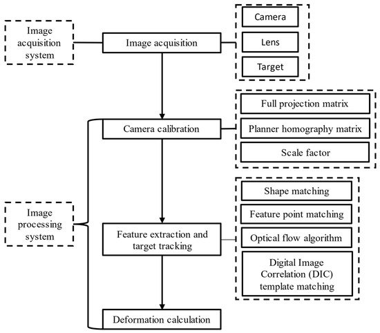
Figure 1.
Process of deformation monitoring based on computer vision.
3.1. Image Acquisition
Image acquisition includes these steps: (1) determine the position to be monitored; (2) arrange artificial targets or use natural targets on the measurement points; (3) select an appropriate camera and lens; (4) assemble the camera lens and set it firmly on a relatively stationary object; (5) aim at the target and acquire images.3.2. Camera Calibration
Camera calibration [40] is the process of determining a set of camera parameters which associate real points with points in the image. Camera parameters can be divided into internal parameters and external parameters: internal parameters define the geometric and optical characteristics of the camera, while external parameters describe the rotation and translation of the image coordinate system relative to a predefined global coordinate system [41]. In order to obtain the structural displacement from the captured video image, it is necessary to establish the transformation relationship from physical coordinates to pixel coordinates. The common coordinate conversion methods are full projection matrix, planar homography matrix, and scale factor.3.2.1. Full Projection Matrix
The full projection matrix transformation reflects the whole projection transformation process from 3D object to 2D image plane. The camera internal matrix and external matrix can be obtained by observing a calibration board, which can be used to eliminate image distortion and has a high accuracy [42]. Commonly used calibration boards include checkerboard [43] and dot lattice [44]. Figure 2a shows the relationship between the camera coordinate system, the image coordinate system and the world coordinate system. A point T (X, Y, Z) in the real 3D world appears at the position t (x, y) in the image coordinate system after the projection transformation (where the origin of the coordinates is P). The relationship between the pixel coordinate system and the image coordinate system is shown in Figure 2b. Therefore, the equation for converting a point from a coordinate in the 3D world coordinate system to a coordinate in the pixel coordinate system is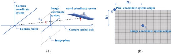
Figure 2. (a) Relationship among the camera coordinate system, the image coordinate system, and the world coordinate system; and (b) Relationship between the pixel coordinate system and the image coordinate system.
3.2.2. Planar Homography Matrix
In practical engineering applications, the above calibration process is relatively complex. To simplify the process, Equation (1) can be expressed3.2.3. Scale Factor
The scale factor (S) provides a simple and practical calibration method. As shown in Figure 3a, when the camera optical axis is perpendicular to the surface of the object, S (unit: mm/pixel) can be obtained based on the internal parameters of the camera (focal length, pixel size) and the external parameters of the camera and the surface of the object (measurement distance) in a simplified calculationfrom the simplified formula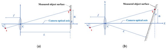
Figure 3. Scaling factor calibration method. (a) Camera optical axis orthogonal to measured object surface; (b) Camera optical axis intersecting obliquely with measured object surface.