Cosmology can serve to determine Neutrino's properties

Cosmology can serve to determine Neutrino's properties: Comparison

Please note this is a comparison between Version 2 by Ziad Sakr and Version 4 by Ziad Sakr.

Neutrino particles have been found, due to their non-interacting, almost-vanishing mass, and relativistic nature, as being suitable to hold roles in many phenomena in nature, which have made them attract a large interest among the scientific community. In particular, on the cosmological level, the neutrino is one of the few components whose contribution to the Universe energy budget changes with its expansion, from being part of the radiation to that of the matter density, with implications on the expansion of the background or the growth of large-scale structures. It has also the feature of being abundantly present since the Universe’s early beginning, participating by then to the different phases of its evolution, which allows us to constrain its main properties such as its mass and number of species by any of the known cosmological observables.

neutrinos
cosmological observables
cosmological parameters

Since their introduction as a solution to the deficit of energy budget in beta decay processes [1], neutrino particles attention has grown bigger with the recent discovery of neutrino oscillations in solar and atmospheric measurements as an evidence of having, though very small, a non-zero mass [2]. Besides the implications on cosmology and astrophysics, this discovery had a consequence on the level of the standard model (SM) of particles, as it calls for a modification of the latter.

However, the value of their mass has not been well determined yet, and only higher limits have been derived. Moreover, the sign of the largest mass splitting, the one governing atmospheric transitions, is still unknown, which leaves open two possibilities for the neutrino masses ordering, corresponding to what is called the normal hierarchy, in which the atmospheric splitting is positive, and the inverted hierarchy, in which it is negative [1].

Other unknowns are still present for the neutrino particle, among them the value of a possible CP-violating phase in the neutrino-mixing matrix, and the Dirac or Majorana nature of the neutrino, i.e., whether or not the neutrino and its antiparticles are the same [1].

There are, however, different ways to constrain the absolute total neutrino masses scale, starting from terrestrial or laboratory experiments, where we can use energy and momentum conservation to determine the mass of the quantity involved from their kinematic effects on the electrons produced in the β decay of nuclei. This could be obtained practically from monitoring distortions in the energy spectrum produced using either holmium 163 isotopes, where the decay energy is measured with micro-calorimeters, or by exploiting the single-β decay of molecular tritium [1].

Neutrinos could also be detected when succeeding in observing some astrophysical cataclysmic events, such as supernova explosions or mergers between two compact objects, for instance two neutron stars or a neutron star and a black hole. Such events usually lead to a compression for high-density volumes so that the proton and electrons combine and release neutrinos that carry most of the energy of the collapse [3]. They also play a role in cooling the torus around the central remnant of a massive neutron star, a black hole, or the nucleosynthesis of heavy nuclei through r-processes in SN remnants. If the event is monitored in its whole duration, it is possible to obtain information on the neutrino velocity since its energy could be measured, hence its mass.

On the cosmological level, the neutrino is one of the few components whose contribution to the energy budget changes its contribution with the Universe’s expansion, from being part of the radiation to that of the matter density, with implications on the expansion of the background or the growth of large-scale structures [4]. It has also the feature of being abundantly present since the Universe’s early beginning, participating by then to the different phases of its evolution, which allows us to constrain it by any of the known cosmological observables, such as the cosmic microwave radiation spectrum (CMB), the imprint left from the early baryonic acoustic oscillations (BAO) on the galaxy’s distribution, the geometric distance from the light curve of the supernova or the more direct growth of structure probes, such as the shear power spectrum from weak-lensed galaxies by matter densities, or the abundance of the clusters or galaxies.

1. Introduction

Since their introduction as a solution to the deficit of energy budget in beta decay processes, neutrino particles attention has grown bigger with the recent discovery of neutrino oscillations in solar and atmospheric measurements as an evidence of having, though very small, a non-zero mass. Besides the implications on cosmology and astrophysics, this discovery had a consequence on the level of the standard model (SM) of particles, as it calls for a modification of the latter. However, the value of their mass has not been well determined yet, and only higher limits have been derived. Moreover, the sign of the largest mass splitting, the one governing atmospheric transitions, is still unknown, which leaves open two possibilities for the neutrino masses ordering, corresponding to what is called the normal hierarchy, in which the atmospheric splitting is positive, and the inverted hierarchy, in which it is negative. Other unknowns are still present for the neutrino particle, among them the value of a possible CP-violating phase in the neutrino-mixing matrix, and the Dirac or Majorana nature of the neutrino, i.e., whether or not the neutrino and its antiparticles are the same. There are, however, different ways to constrain the absolute total neutrino masses scale, starting from terrestrial or laboratory experiments, where the researchers can use energy and momentum conservation to determine the mass of the quantity involved from their kinematic effects on the electrons produced in the β decay of nuclei. This could be obtained practically from monitoring distortions in the energy spectrum produced using either holmium 163 isotopes, where the decay energy is measured with micro-calorimeters, or by exploiting the single-β decay of molecular tritium.

Neutrinos could also be detected when succeeding in observing some astrophysical cataclysmic events, such as supernova explosions or mergers between two compact objects, for instance two neutron stars or a neutron star and a black hole. Such events usually lead to a compression for high-density volumes so that the proton and electrons combine and release neutrinos that carry most of the energy of the collapse. They also play a role in cooling the torus around the central remnant of a massive neutron star, a black hole, or the nucleosynthesis of heavy nuclei through r-processes in SN remnants. If the event is monitored in its whole duration, it is possible to obtain information on the neutrino velocity since its energy could be measured, hence its mass.

On the cosmological level, the neutrino is one of the few components whose contribution to the energy budget changes its contribution with the Universe’s expansion, from being part of the radiation to that of the matter density, with implications on the expansion of the background or the growth of large-scale structures. It has also the feature of being abundantly present since the Universe’s early beginning, participating by then to the different phases of its evolution, which allows us to constrain it by any of the known cosmological observables, such as the cosmic microwave radiation spectrum (CMB), the imprint left from the early baryonic acoustic oscillations (BAO) on the galaxy’s distribution, the geometric distance from the light curve of the supernova or the more direct growth of structure probes, such as the shear power spectrum from weak-lensed galaxies by matter densities, or the abundance of the clusters or galaxies.

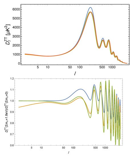
2. Neutrino Effects on the CMB Power Spectrum

Neutrinos will have different effects on the CMB spectrum. ThWe researchers remind that the latter anisotropies are encoded in the power spectrum2 coefficients Cℓs, i.e., the coefficients of the expansion in the Legendre polynomials $P_{ℓ} (x)$ of the two-point angular correlation function on the angular scales $θ = π / ℓ$ . In the case of the temperature angular fluctuations

δ T ( n ^ ) T ¯

\frac{δ T (\hat{n})}{\bar{T}}

in CMB, it is expressed as:

(120)

More theoretically, and to gain some further insights, thwe researchers describe how temperature fluctuations measured from the CMB are related to radiation-matter inhomogeneities interactions, by the following approximate formula from references ^[1][5], assuming recombination happened fast near the surface of the last scattering, a condition allowing to separate source evolution calculations from geometrical complexity:

(21)

where the first term of the right-hand side is the temperature anisotropy in the point of the last scattering surface, the second term comes from the gravitational shift of the photons traveling along in gravitational potential fluctuations known as the early Sachs–Wolf (SW) effect. It is followed by the correction to this temperature coming from the conventional Doppler caused by the velocity of the baryon–photon fluid. The last term is relative to the integrated Sachs–Wolfe (ISW) effect. It describes how the CMB angular power spectrum is affected on large scales when passing through varying potentials on its way towards the observer.

The shape of the observed power spectra is the result of the processes taking place in the primordial plasma around the time of recombination. Therefore, thwe researchers observe a series of peaks and troughs in the temperature power spectrum, corresponding to oscillation modes that were caught at an extreme of compression or rarefaction (the peaks), or exactly in phase with the background (the troughs). The typical scale of the oscillations is set by the sound horizon at the recombination

r_{s} (z_{r e c}) = \int_{z_{r e c}}^{\infty} \frac{c_{s} (z) d z}{H (z)}

, i.e., the distance traveled by an acoustic wave (

c_{s}

being the sound speed) from some very early time until

z_{r e c}

, the redshift of recombination and the presence of baryons, which shifts the zero of the oscillations, introducing an asymmetry between even and odd peaks. Finally, the peak structure is further modulated by an exponential suppression, due to the Silk damping of photon perturbations. The height of the first peak also depends on the redshift of equivalence

z_{e q}

Equation (310) (which sets the enhancement in power due to the early SW effect). Thus, the acoustic peaks hold most the information by their amplitudes and position functions of the angular separations in the CMB anisotropies.

1 + z e q = Ω c + Ω b Ω γ 1 + 7 8 4 11 4 / 3 N eff ,

(3)

Different effects related to the neutrinos’ density value, effective number, or their transition from relativistic to massive particles, are then induced.

From being part of the radiation budget at the recombination epoch, the neutrino will change the expansion and impact the angular diameter distance (in the flat Universe for simplicity) to the last scattering surface

r A ( z r e c ) = ∫ 0 z r e c d z H ( z ) ( 1 + z )

r_{A} (z_{r e c}) = \int_{0}^{z_{r e c}} \frac{d z}{H (z) (1 + z)}

, controlling the overall position of the CMB spectrum peaks in multipole space. This is degenerate with the matter density effect, including that on the slope of the low-ℓ tail of the CMB spectrum, due to the late-integrated Sachs–Wolfe (ISW) effect, but also with the redshift radiation-matter equality time

z_{e q}

that impacts the early SW effect. Figure 13 illustrates some of these effects, where the model in blue has a smaller

z_{e q}

with respect to the reference; the models in yellow and green have a larger

θ_{s}

(s for scattering); in addition, the yellow model also has a smaller

z_{Λ}

(redshift of transition to dark energy domination over matter).

Figure 13. Top: CMB TT power spectra for different values of

\sum m_{ν}

, taken from reference ^[2][6]. The quantity on the vertical axis is

D_{ℓ}^{T T} \equiv ℓ (ℓ + 1) C_{ℓ}^{T T} / 2 π

. The red curve is a cosmological model with

\sum m_{ν} = 0.06

eV and all other parameters fixed to the Planck best-fit. The other curves are for models with

\sum m_{ν} = 1.8

eV, in which the curvature is kept vanishing by changing h (green),

Ω_{Λ}

(yellow), or

Ω_{c} h^{2}

(blue). Bottom: Ratio between the models with

\sum m_{ν} = 1.8

eV and the reference model.

ThWe researchers aalso note another consequence of a change in the neutrino density, coming from different wavelengths entering at different epochs with changes in their time of travel following that of the expansion rate function of neutrino density. This impacts the early SW effect, which would stretch the position of the peaks. More neutrinos also imply stronger gravitational interactions between photons and free-streaming species before decoupling, which is important for scales that have just crossed the Hubble scale during the radiation domination epoch, resulting in a small shift and damping of the acoustic peak (“baryon drag” effect). This will also affect the “Silk” damping of the CMB anisotropies, as a higher

N_{eff}

changes the scale of this damping relative to the scale of the sound horizon at decoupling, which appears as a shift in the damping envelope of high peaks relative to the position of the first peak.

More secondary effects would also be generated from the neutrinos, later becoming non-relativistic and massive when, according to Equation (17), they escape the halo’s potential and slow the growth of the formation of large-scale structures, thus affecting the late ISW effect at low ell but also modifying the lensing from the large-scale structures on the multipoles. ThWe researchers eend by a final subtle effect, when neutrinos, becoming non-relativistic, reduce the time variation of the gravitational potential inside the Hubble radius, affecting the photon temperature through the early SW effect, leading to a depletion in the temperature spectrum.

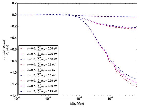
32. Effects of Neutrino on Large-Scale Structure Formation

Before thwe researchers present the effect of massive neutrinos on large-scale structure formation, the researchers we first mention their impact on the baryonic acoustic oscillation (BAO) signal or the relic signature of the first peak in CMB, showing in-galaxy clustering through an enhancement in the amplitude of their angular correlation function of the angular distance

r_{A} (z)

. As thwe researchers shshall see later, this distance probe at relatively much lower redshift than that of the epoch of recombination of the CMB (but measured at different times), could, through the contribution of the neutrino’s density to the angular distance

r_{A} (z)

, break the matter density or Hubble constant’s total neutrino masses’ degeneracy and thus allow the first peak of the CMB spectrum to put stronger constraints on the neutrino’s density. Other geometric measurements such as those coming from the luminosity distance of SNIa can play the same role, as well as direct measurements of

H_{0}

that rely on local distance indicators that are little or not-at-all dependent on the underlying cosmological model.

ThWe researchers move next to the matter domination epoch, where large-scale structure (LSS) formation mainly happens. There, the neutrino’s effect would be to mainly suppress growth rate, while its effect on the matter–radation redshift value will impact the LSS power spectrum formation, and from changes in the time density waves enter the gravitational horizon scale.

As an example to the influence of the first effect, the reswearchers discuss the impact of neutrino density variation on the LSS power spectrum. Most LSS-related observables have the power spectrum as one of their ingredients, among them for example, the clustering of matter at large scales, a powerful probe of cosmology that can be described in terms of the two-point correlation function, or, equivalently, of

P_{m}

, the power spectrum of matter density fluctuations:

(422)

where

δ m ( k → , z )

δ_{m} (\vec{k}, z)

is the Fourier transform of the matter density perturbation at redshift z. Note that, contrarily to the CMB, thwe researchers are are bound to observe at a single redshift (that of recombination), that the matter power spectrum can, in principle, be measured at different times in the cosmic history, thus allowing for a tomographic and cross-correlations analysis resulting in strong constraints in parameters, such as the total neutrino masses, as we see next.

So, a first consequence of massive neutrino free-streaming is that, below the free-streaming scale, there is a smaller amount of matter that can cluster. This results in an overall suppression of the power spectrum at small scales, with respect to the neutrinoless case. Secondly, similar to what thwe researchers observed in CMB interactions, subhorizon perturbations in the non-relativistic (i.e., cold dark matter and baryons) components grow more slowly. In fact, while in a perfectly matter-dominated Universe the gravitational potential is constant and the matter perturbation grows linearly with the scale factor

δ m ∝ a

δ_{m} \propto a

with

a = ( 1 + z ) − 1

a = {(1 + z)}^{- 1}

, in a mixed-matter–radation Universe, the gravitational potential decays slowly inside the horizon. Below the free-streaming scale, neutrinos effectively behave as radiation; then, in the limit in which the neutrino fraction

f ν = Ω ν / Ω m

f_{ν} = Ω_{ν} / Ω_{m}

is small, one has for

k ≫ k fs

k ≫ k_{fs}

(523)

while

δ m ∝ a

δ_{m} \propto a

is for

k ≪ k fs

k ≪ k_{fs}

These two effects can be approximated by the ratio

P m ( k ≫ k fs , f ν ) / P m ( k ≫ k fs , f ν = 0 ) ≃ 1 − 8 f ν

P_{m} (k ≫ k_{fs}, f_{ν}) / P_{m} (k ≫ k_{fs}, f_{ν} = 0) ≃ 1 - 8 f_{ν}

^[3][7]. This is illustrated in Figure 24, where thwe researchers observe higher depletion with the increment of the mass of neutrinos while showing also a bigger effect at low masses with respect to high redshifts. Note that hierarchical neutrinos will each modify the power spectrum at slightly different free-streaming scales due to their individual masses, which allow to constrain hierarchy in principle, though it will be very difficult to disentangle these subtle signatures from the noise and the variance in the data.

Figure 24. Illustrating the depletion of the linear matter power spectrum ( $P_{k}$ ) for different neutrino masses by showing the residual of the massive neutrinos

P_{k}

to the massless ones for different redshifts.

As a consequence, thwe researchers will be able to use an observable at slightly higher redshift than BAO as a stronger probe to the neutrinos’ mass: the forest of small clustering of matter detected by the Lyman-

α

signal that are very sensitive to the free streaming of neutrinos.

Another consequence from a larger neutrino mass and less clustering on small scales is to decrease lensing by affecting the path of the photons coming from distant sources, since those photons will be deflected by the gravitational potentials along the line of sight. For CMB, this modifies the anisotropy pattern by mixing photons that come from different directions. In the temperature and polarization power spectra, the result is that the peaks and troughs at high ℓs are sharper. Additionally, lensing, being a non-linear effect, creates some amount of non-Gaussianity in the anisotropy pattern that can be detected and measured by looking at higher-order correlations in the CMB, offering another independent probe through the measured four-point correlation function referred to by the CMB lensing power spectrum. Neutrino mass is here constrained by its impact on the smoothing of the latter power spectrum at high ℓs. The power spectrum of the lensing potential is also detected from the measurements of the lensing-induced ellipticity of background galaxies with an effect more constraining than CMB when all the LSS lensing systematics are further reduced because it can be probed at different epochs, allowing a tomographic fix of the neutrino masses.

ThWe researchers shshall show later the latest constraints from CMB, BAO, SN, and direct measurements of $H_{0}$ and LSS, each alone or in combination, but thwe researchers note here that the CMB and BAO seems to prefer a null or very low value for the neutrinos’ mass in difference with higher ones coming from structure formation or lensing.

On the non-linear effect, it has been shown by Costanzi et al. ^[4][8] and Castorina et al. ^[5][9] that the determination of the non-linear matter power spectrum or the matter fluctuation parameter

σ_{8}

with massive neutrinos agrees with simulations if the researchers we only take the cdm+baryon power spectrum in a halo model approach to construct the non-linear power spectrum, or if the researchers we want to compute

σ_{8}

43. Neutrinos Mass and Number Constraints from Cosmological Observables

ThWe researchers hhave seen the neutrino mass and number of species impact on cosmological observables and the possibility to use them to constrain neutrino properties. However, being involved in most of the physical processes, neutrinos effect could degenerate with other cosmological parameters, such as, for example, the matter density parameter’s impact on the growth of structure or the universe’s expansion, along with the Hubble constant. This could weaken the constraints from a single probe unless the researchers we combine different ones to break the degeneracies and tighten by then the bounds on the neutrino properties. As an example, Di Valentino (2021) ^[6][10], using the latest determinations of the growth rate parameter, along with CMB and a BAO measurements from galaxy clustering, set the upper limit to ∑ m ν < 0.09 eV at a 95% confidence level.

However, with the current observations, even if thwe researchers ccombine most of the available datasets, there will still be room for more than 10% inaccuracy on its mass or number of species.

Below, thwe researchers ccompile most of the current upper bounds in one Figure 35 to better picture the status and compare the capabilities of the different probes or their combinations in constraining properties on the neutrino masses.

neutrino masses current bounds

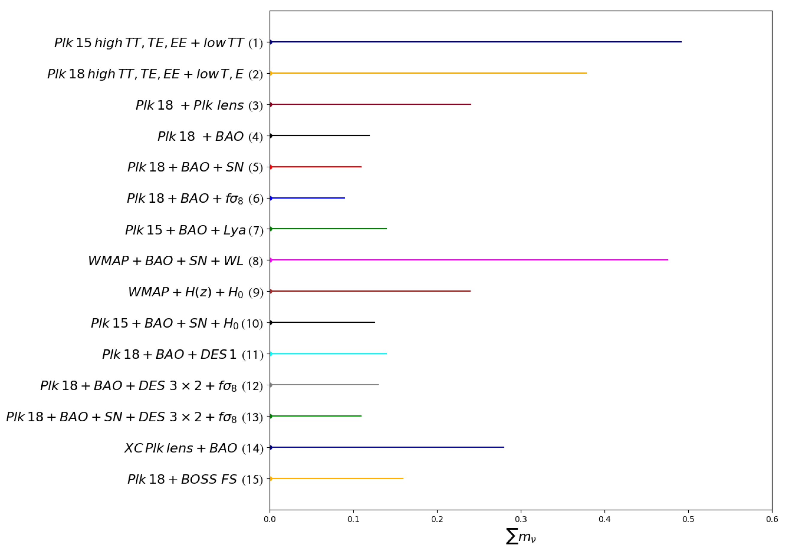
Figure 35. Total neutrino masses upper bounds at the 95% confidence level from different combinations of currently available cosmological probes.

Total neutrino masses upper bounds at the 95% confidence level from different combinations of currently available cosmological probes (see references here)

That is why the next generation of surveys, such as Euclid ^[7][11], LSST-Rubin ^[8][12], WFIRST-Roman ^[9][13], SKA ^[10][14], CMB-S4 ^[11][15], or DESI ^[12][16], with one or even two orders of magnitude higher in terms of the density of the observations or depth in the redshift, are necessary to reach the evidence for the mass detection of the number of species beyond the five σ required to claim a discovery. However, this also might not be sufficient unless thwe researchers include further surveys that are able to constrain the last degeneracy that the upcoming surveys could not break, i.e., the optical depth, which degenerate with the amplitude of the power spectrum or the polarization present in the corresponding spectrum from CMB and, that by using deeper redshift surveys, are able to reach the epoch of reionization, such as Litebird ^[13][17] or CORE ^[14][18], and are also spanning most of the fraction of the sky to limit to a the maximum the cosmic variance, with the latter being one of the main limits to the use of large-scale modes in different-measured power spectrums to further constrain cosmological parameters as well as neutrino masses.

Below, thwe researchers ccompile most of the forescasted bounds in one Figure 46 to better picture the status and capabilities of the upcoming probes and their combinations in constraining properties on the neutrino mass.

Neutrino masses forecasted bounds

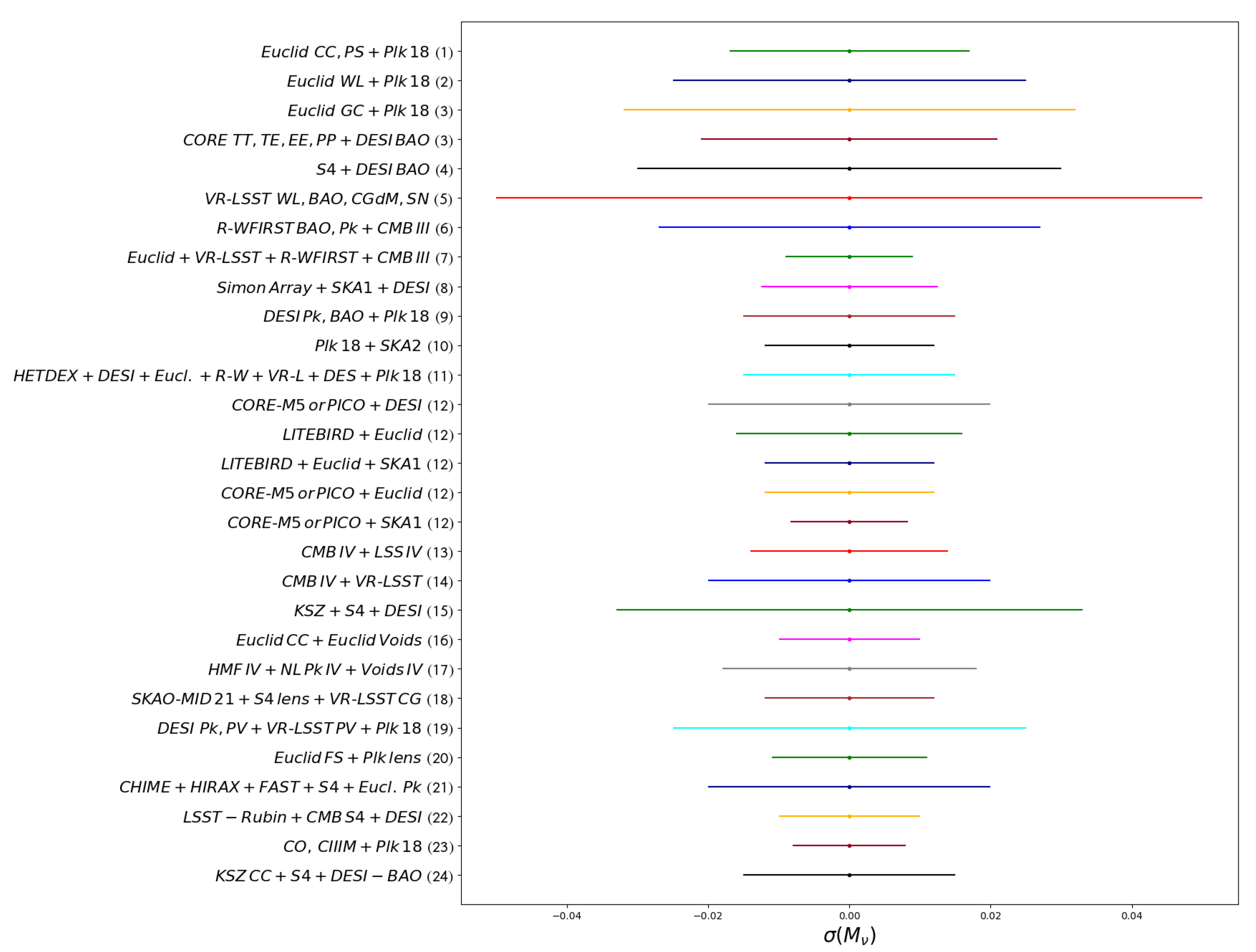
Figure 46. Neutrino uncertainty mass bounds at 68% confidence level from different combinations of upcoming cosmological experiments.

Neutrino uncertainty mass bounds at 68% confidence level from different combinations of upcoming cosmological experiments (see references here).

Still, these will act on the total mass of the neutrino species while the hierarchy or the individual mass of each of the neutrino’s flavors will have to wait until surveys with a capacity beyond Stage IV to be detected, or else, combining upcoming surveys with future terrestrial and astrophysical experiments to limit the allowed space of variation of neutrino masses ^[15][19].