AI and General movements (GMs)

AI and General movements (GMs): Comparison

Please note this is a comparison between Version 1 by Muhammad Tausif Irshad and Version 3 by Conner Chen.

General movements (GMs) are spontaneous movements of infants up to five months post-term involving the whole body varying in sequence, speed, and amplitude. The assessment of GMs has shown its importance for identifying infants at risk for neuromotor deficits, especially for the detection of cerebral palsy. As the assessment is based on videos of the infant that are rated by trained professionals, the method is time-consuming and expensive. Therefore, approaches based on Artificial Intelligence have gained significantly increased attention in the last years.

general movement assessment
fidgety movements
cerebral palsy
motion sensors
visual sensors
multimodal sensing
physical activity assessment
machine learning
artificial neural network

1. Sensor Modalities Used for General Movement Assessment

The advancement in sensor technology facilitates the automatic monitoring of infants’ movements. Hence, a system using visual or motion sensors can be useful to track these movements to diagnose motor impairments at early stages. This section briefly describes the sensor modalities used in the reviewed studies. Table 1 specifies the sensor modalities used by a particular GMA study.

Table 1. The list of sensors used for the assessment of general movements (GMs) and fidgety movements (FMs).

	Meinecke et al. ^[1]	Rahmati et al. ^[2]	Adde et al. ^[3]	Raghuram et al. ^[4]	Stahl et al. ^[5]	Schmidt et al. ^[6]	Ihlen et al. ^[7]	Gao et al. ^[8]	Machireddy et al. ^[9]	McCay et al. ^[10]	Orlandi et al. ^[11]	Olsen et al. ^[12]	Singh and Patterson ^[13]	Dai et al. ^[14]	Heinze et al. ^[15]	Gravem et al. ^[16]	Rahmati et al. ^[17]	Tsuji et al. ^[18]	Philippi et al. ^[19]	Karch et al. ^[20]	Adde et al. ^[21]	Fan et al. ^[22]	McCay et al. ^[23]
Modalities	Meinecke et al. ^[1]	Rahmati et al. ^[2]	Adde et al. ^[3]	Raghuram et al. ^[4]	Stahl et al. ^[5]	Schmidt et al. ^[6]	Ihlen et al. ^[7]	Gao et al. ^[8]	Machireddy et al. ^[9]	McCay et al. ^[10]	Orlandi et al. ^[11]	Olsen et al. ^[12]	Singh and Patterson ^[13]	Dai et al. ^[14]	Heinze et al. ^[15]	Gravem et al. ^[16]	Rahmati et al. ^[17]	Tsuji et al. ^[18]	Philippi et al. ^[19]	Karch et al. ^[20]	Adde et al. ^[21]	Fan et al. ^[22]	McCay et al. ^[23]
RGB Camera		X	X	X	X	X	X		X	X	X			X			X	X	X		X		X
Vicon System	X
Microsoft Kinect							X			X		X											X
Accelerometer													X		X	X						X
IMU								X	X
EMTS		X															X		X	X

Dear author, the following contents are excerpts from your papers. They are editable.

Movements of the human body look very simple but consist of complex coordination systems, subsystems, and monitoring pathways. Any disorder in the coordination system like progressive neuromuscular disorders, injuries to the brain, and genetic disorders can create problems in movement and posture. For example, cerebral palsy (CP) describes a group of disorders of lifelong physical disability caused by a non-progressive brain injury or lesion acquired during the antenatal, perinatal, or early postnatal period [1]. The severity, patterns of motor involvement, and associated impairments, such as communication, intellectual ability, and epilepsy, vary widely and persist across the life course [2]. In addition, neonatal mortality has decreased in preterm infants in the past decade, extremely preterm infants (born at <27 gestational weeks) remain at the highest risk for neonatal morbidity and the occurrence of CP [3]. Therefore, the prevalence of CP has remained stable over the last forty years at 2–3 per 1000 live births in countries with a developed health care system.

At present, there are no uniform clinical procedures for the prediction of motor impairments like CP in high-risk infants and the recognition of those at the highest risk generally requires the combination of clinical history, various clinical assessments and expertise of the observer [4]. Some studies, e.g., [5,6,7], have exposed the fact that early recognition of motor impairment leads to early interventions that might reduce the severity of the motor impairment and the restrictions in daily activities [8].

Prechtl presented the General Movements Assessment (GMA) as a valuable tool for the prediction of cerebral palsy in high-risk infants [9,10]. General movements (GMs) are spontaneous movements of infants up to five months post-term involving the whole body. The movements vary in sequence, speed, and amplitude. Depending on the infant’s age, one distinguishes between the general movements (GMs) (preterm general movements (∼28–36/38 gestational weeks) or term/writhing movements (36/38–46/52 gestational weeks)), and the fidgety movements (FMs) (46/50–55/60 gestational weeks) [9]. Next to normal GMs and normal FMs (F+ or F++), one distinguishes between poor repertoire GMs (PR) with a monotonous sequence of movements and reduced variance in speed and amplitude of movements, cramped synchronized GMs (CS) which appear stiff with bilateral contraction and relaxation of the legs and the abdominal wall, and chaotic GMs (Ch) which appear jerky, rowing, fast, and have a large amplitude. The non-normal FMs comprise abnormal FMs (AF) with large amplitude, fast and jerky movements, as well as the absence of FMs (F−). Showing cramped synchronized or chaotic GMs around term or the absence of fidgety movements (F−) at 3 to 5 months post-term have an excellent predictive value for cerebral palsy [11,12]. However, the assessment is based on videos of the infant that are rated by trained professionals, therefore, the method is time-consuming and expensive.

As a result of the nominal use of GMA in neonatal follow-up programs, several studies have tried to automate this method. These studies are based on either indirect sensing using visual sensors (2D or 3D video) [7,13,14,15,16,17,18,19,20,21,22,23,24,24], direct sensing using motion sensors [25,26,27,28,29,30,31], or both [32,33,34]. They have shown excellent results, however, they lack full automation and also have several fundamental limitations. First, all the studies are either based on a small number of subjects or a fewer number of data samples with respect to CP [7,18,19,20,25,26,27,32,34]. It is also not clear if the prediction model in these studies has external validity for high-risk infants. Second, the research work in some studies is based on convenience samples that do not reflect the usual clinical cohorts. Third, the movement features used in previous studies lack generality due to less number of subjects and examples. Lastly, all the reviews, except [17,20,23,24,35,36], are not using state-of-the-art Deep Learning (DL) algorithms to automate the GMA process. The DL algorithms are popular approaches of Artificial Intelligence (AI) which not only provide a generalized solution but also perform well for accurate detection of the classes in visual and time-series data. Therefore, an end-to-end system is needed to analyze the infant’s movements in the early infancy.

There are some related review articles for monitoring body movements of infants using sensor technology. Chen et al. [37] outlines the wearable sensor systems for monitoring body movements of neonates apart from visual sensors and state-of-the-art AI algorithms for the development of an automated end-to-end system. Zhu et al. [38] present a broad overview of wearable sensors intending to measure various types of physiological signals of infants. The authors in [39] discuss state-of-the-art movement recognition technology for assessing spontaneous general movements in high-risk infants, however, they do not focus on the design and development of the system. They discuss the wearable and visual sensors averagely. Zhang [40] review machine learning methods in cerebral palsy research and evaluates algorithms in movement assessment for CP prediction.

The primary objective of this article is to systematically analyze and discuss the main design features of all existing technological approaches trying to classify the general movements of infants and explain the methodological reasons for their limited practical performance and classification rates. The main contributions of this paper can be summarized as follows:

RGB Camera records the color information at the time of exposure by evaluating the spectrum of colors into three channels, i.e., red, green, and blue. They are easily available, portable, and suitable for continuous assessment of infants in clinics or at home due to their contact-less nature comparing with other modalities. Various motion estimation methods for example, Optical Flow, Motion Image, can be used for RGB videos.
We present a structured review of the current technological approaches that detect general movements and/or fidgety movements, and categorize them according to the AI techniques they use. We slice up these approaches into three vital categories: visual sensor-based, motion sensor-based, and multimodal (fusion of visual and motion sensory data).

Vicon System is an optoelectronic motion capture system based on several high-resolution cameras and reflective markers. These markers are attached to specific, well-defined points of the body. As a result of body movement, infrared light reflects into the camera lens and hits a light-sensitive lamina forming a video signal. It collects visual and depth information of the scene ^[24].
We categorize and present a summary of the sensor technology and classification algorithms used in the existing GMA approaches.

Microsoft Kinect
sensor consists of several state-of-the-art sensing hardware such as RGB camera, depth sensor (RGB-D), and microphone array that helps to collect the audio and video data for 3D motion capture, facial, and voice recognition. It has been popularly used in research fields related to object tracking and recognition, human activity recognition (HAR), gesture recognition, speech recognition, and body skeleton detection. ^[25].
We also present a comparative analysis of reviewed AI-based GMA approaches with respect to input-sample size, type of features, and classification rate.

Accelerometers are sensing devices that can evaluate the acceleration of moving objects and reveal the frequency and intensity of human movements. They have been commonly used to monitor movement disorders, detect falls, and classify activities like sitting, walking, standing, and lying in HAR studies. Due to small size and low-price, they have been commonly fashioned in wearable technologies for continuous and long-term monitoring ^[26][27].

Inertial Measurement Unit (IMU) is a sensory device that provides the direct measurement of multi-axis accelerometers, gyroscopes, and sometimes other sensors for human motion tracking and analysis. They can also be integrated in wearable devices for long term monitoring of daily activities which can be helpful to assess the physical health of a person ^[28]

2. Classification Algorithms Applied for General Movement Assessment

In machine learning, classification and regression algorithms are used to predict results based upon input data. A classification categorizes the data into predefined classes, whereas regression estimates an outcome from a set of input data. These algorithms are implemented in two phases—training and testing. In each of these phases, the raw data are acquired by sensors. After pre-processing the data, suitable features are extracted to build feature vectors. The feature vectors can be split into train and test datasets. In the training phase, the train dataset is used to train a model. In the testing phase, the trained model is used to predict the results of feature vectors belonging to the test dataset. Finally, the performance of the model is evaluated using different matrices on the test data. Figure 1 shows the essential stages of classification.

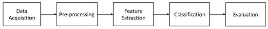
Figure 1. This figure shows necessary steps to solve a classification problem.

Sensors used in data acquisition process for the assessment of GM and FM studies are shown in Table 1. Features extraction process is out of the scope of our topic.

In general, a classification algorithm evaluates the input features to make a decision or diagnosis. The selection of the algorithm depends on many factors, for example, type of data, size of data, and available resources to process the data. This section provides the description of classification algorithms used in GMA studies for the discrimination of infant’s movements or impairments.

Naive Bayes (NB) belongs to the group of probabilistic classifiers based on implementing the Bayes’ theorem with the simple assumption of conditional independence that the value of a feature is independent of the value of any other feature, and each feature contributes independently to the probability of a class. NB combines the independent feature model to predict a class with a common decision rule known as maximum likelihood estimation or MLE rule. Despite their simplicity, NB classifiers performed well on many real-world datasets such as spam filtering, document classification, and medical diagnosis. They are simple to implement, need a small amount to training data, can be very fast in prediction as compared to most well-known methods ^[31].

Linear Discriminant Analysis (LDA) is used to identify a linear combination of features that splits two or more classes. The subsequent combination can be used as a linear classifier or dimensionality reduction step before the classification phase. LDA is correlated to principal component analysis (PCA), which also attempts to find a linear combination of best features ^[32]. However, PCA reduces the dimensions by focusing on the variation in data and cannot form any difference in classes. In contrast, it maximizes the between-class variance to the within-class variance to form maximum separable classes ^[33].

Quadratic Discriminant Analysis (QDA) is a supervised learning algorithm which assumes that each class has a Gaussian distribution. It helps to perform non-linear discriminant analysis and believes that each class has a separate covariance matrix. Moreover, It has some similarities with LDA, but it cannot be used as a dimensionality reduction technique .

^[^34].

Logistic Regression (LR) explores the correlation among the independent features and a categorical dependent class labels to find the likelihood of an event by fitting data to the logistic curve. A multinomial logistic regression can be used if the class labels consist of more than two classes. It works differently from the linear regression, which fits the line with the least square, and output continuous value instead of a class label ^[35].

Support Vector Machine (SVM) is a supervised learning algorithm that analyzes the data for both classification and regression problems. It creates a hyperplane in high dimensional feature space to precisely separate the training data with maximum margin, which gives confidence that new data could be classified more accurately. In addition to linear classification, SVM can also perform non-linear classification using kernels ^[36].

Electromagnetic Tracking System (EMTS) provides the position and orientation quantities of the miniaturized sensors for instantaneous tracking of probes, scopes, and instruments. Sensors entirely track the inside and outside of the body without any obstruction. It is mostly used in image-guided procedures, navigation, and instrument localization ^[29][30].

K-Nearest Neighbor (KNN)
stores all the training data to classify the test data based on similarity measures. The value of K in the KNN denotes the numbers of the nearest neighbors that can involve in the majority voting process. Choosing the best value of k is called parameter tuning and is vital for better accuracy. Sometimes it is called a lazy learner because it does not learn a discriminative function from the training set. KNN can perform well if the data are noise-free, small in size, and labeled
^[
³⁷^].

Decision Tree (DT) is a simple presentation of a classification process that can be used to determine the class of a given feature vector. Every node of DT is either a decision node or leaf node. A decision node may have two or more branches, while the leaf node represents a classification or decision. In DTs, the prediction starts from the root node by comparing the attribute values and following the branch based on the comparison. The final result of DT is a leaf node that represents the classification of feature vector ^[38].

Random Forest (RF) is an ensemble learning technique that consists of a collection of DTs. Each DT in RF learns from a random sample of training feature vectors (examples) and uses a subset of features when deciding to split a node. The generalization error in RF is highly dependent on the number of trees and the correlation between them. It converges to a limit as the number of trees becomes large ^[39]. To get more accurate results, DTs vote for the most popular class.

AdaBoost (AB) builds a robust classifier to boost the performance by combining several weak classifiers, such as a Decision Tree, with the unweighted feature vectors (training examples) that produce the class labels. In case of any misclassification, it raises the weight of that training data. In sequence, the next classifier is built with different weights and misclassified training data get their weights boosted, and this process is repeated. The predictions from all classifiers are combined (by way of majority vote) to make a final prediction ^[40].

LogitBoost (LB) is an ensemble learning algorithm that is extended from AB to deal with its limitations, for example, sensitivity to noise and outliers ^[41]. It is based on the binomial log-likelihood that modifies the loss function in a linear way. In comparison, AB uses the exponential loss that modifies the loss function exponentially.

XGBoost (XGB) or eXtreme Gradient Boosting is an efficient and scalable use of gradient boosting technique proposed by Friedman et al. ^[41], available as an open-source library. Its success has been widely acknowledged in various machine learning competitions hosted by Kaggle. XGB is highly scalable as compared with ensemble learning techniques such as AB and LB, which is due to several vital algorithmic optimizations. It includes a state-of-the-art tree learning algorithm for managing sparse data, a weighted quantile method to manage instance weights in approximate tree learning—parallel and distributed computing for fast model exploration ^[42].

Log-Linearized Gaussian Mixture Network (LLGMN) is a feed-forward kind of neural network that can estimate a posteriori probability for the classifications. The network contains three layers and the output of the last layer is considered as a posteriori probability of each class. The Log-Linearized Gaussian Mixture formation is integrated in the neural network by learning the weight coefficient allowing the evaluation of the probabilistic distribution of given dataset ^[43].

Convolutional Neural Network (CNN) is a class of ANN, most frequently used to analyze visual imagery. It consists of a sequence of convolution and pooling layers followed by a fully connected neural network. The convolutional layer convolves the input map with k kernels to provide the k-feature map, followed by a nonlinear activation to k-feature map and pooling. The learned features are the input of a fully connected neural network to perform the classification tasks ^[44].

Partial Least Square Regression (PLSR) is a statistical method that uncovers the relationship among two matrices by revealing their co-variance as minimum as feasible, Rahmati et al. ^[17] apply it to predict cerebral palsy in young infants. Here, PLSR uses a small sequence of orthogonal Partial Least Square (PLS) components, specified as a set of weighted averages of the X-variables, where the weights are evaluated to maximize the co-variance with the Y-variables and Y is predicted from X via its PLS components or equivalently ^[17][45].

Discriminative Pattern Discovery (DPD) is a specialized case of Generalized Multiple Instance (GMI) learning, where learner uses a collection of labeled bags containing multiple instances, rather than labeled instances. Its main feature is to solve the weak labeling problem in the GMA study by counting the increment of each instance in order to classify it into three pre-defined classes. Moreover, DPD performs the classification based on the softs core proportion rather than a hard presence/absence criteria as in conventional GMI approaches ^[8].

Prior to continue, it is worth noting that the correct classification of GMs is a difficult task and relies on clinical expertise. While some previous (machine learning) studies evaluated the ground truth of their data by introducing trained GMA experts, some recognized ambiguous, arbitrary, or incorrect classification or did not present detailed information about the realized process. In order to provide an objective overview, we nevertheless indicate the classes and terms specified in the papers and highlight if the classification was not carried out properly. Moreover, this article does not talk about preprocessing operations, for example (image enhancement, noise attenuation, finding the region of interest, etc.), since they fall outside from the scope of this article. In addition, we duly note that understanding this paper requires knowledge of machine learning concepts and performance evaluation techniques of classifiers. An extensive but straightforward explanation of these concepts can be found in [41,42].