Underground sewerage systems (USSs) are a vital part of public infrastructure that contributes to collecting wastewater or stormwater from various sources and conveying it to storage tanks or sewer treatment facilities. A healthy USS with proper functionality can effectively prevent urban waterlogging and play a positive role in the sustainable development of water resources. Since it was first introduced in the 1960s, computer vision (CV) has become a mature technology that is used to realize promising automation for sewer inspections.
- survey
- computer vision
- defect inspection
- condition assessment
- sewer pipes
1. Introduction
1.1. Background
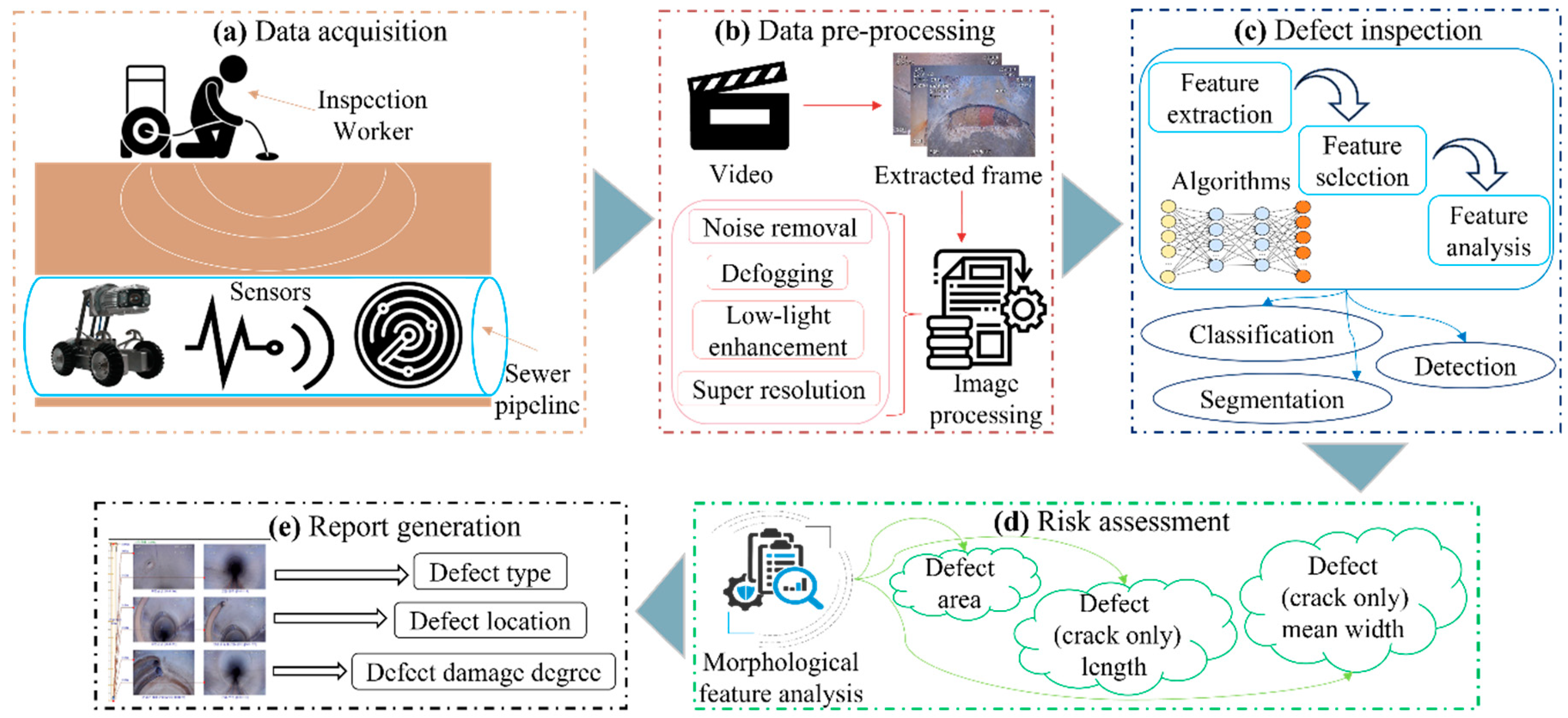
1.2. Defect Inspection Framework

2. Defect Inspection
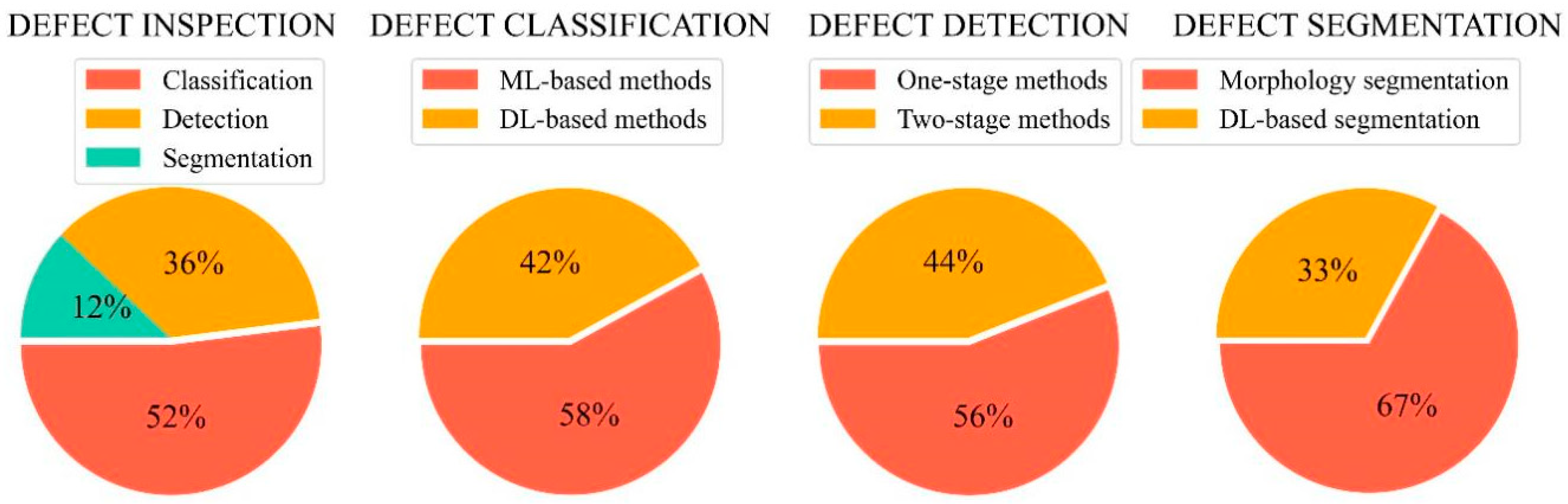
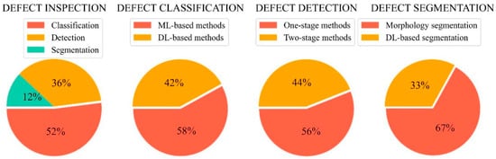
In this section, several classic algorithms are illustrated, and the research tendency is analyzed. Figure 2 provides a brief description of the algorithms in each category. In order to comprehensively analyze these studies, the publication time, title, utilized methodology, advantages, and disadvantages for each study are covered. Moreover, the specific proportion of each inspection algorithm is computed in Figure 3. It is clear that the defect classification accounts for the most significant percentages in all the investigated studies.
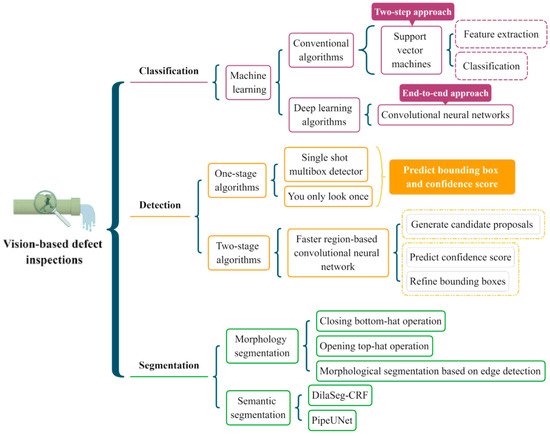
2.1. Defect Classification
Due to the recent advancements in ML, both the scientific community and industry have attempted to apply ML-based pattern recognition in various areas, such as agriculture [14][32], resource management [15][33], and construction [16][34]. At present, many types of defect classification algorithms have been presented for both binary and multi-class classification tasks.2.2. Defect Detection
Rather than the classification algorithms that merely offer each defect a class type, object detection is conducted to locate and classify the objects among the predefined classes using rectangular bounding boxes (BBs) as well as confidence scores (CSs). In recent studies, object detection technology has been increasingly applied in several fields, such as intelligent transportation [17][18][19][75,76,77], smart agriculture [20][21][22][78,79,80], and autonomous construction [23][24][25][81,82,83]. The generic object detection consists of the one-stage approaches and the two-stage approaches. The classic one-stage detectors based on regression include YOLO [26][84], SSD [27][85], CornerNet [28][86], and RetinaNet [29][87]. The two-stage detectors are based on region proposals, including Fast R-CNN [30][88], Faster R-CNN [31][89], and R-FCN [32][90].2.3. Defect Segmentation
Defect segmentation algorithms can predict defect categories and pixel-level location information with exact shapes, which is becoming increasingly significant for the research on sewer condition assessment by re-coding the exact defect attributes and analyzing the specific severity of each defect. The previous segmentation methods were mainly based on mathematical morphology [33][34][112,113]. However, the morphology segmentation approaches were inefficient compared to the DL-based segmentation methods. As a result, the defect segmentation methods based on DL have been recently explored in various fields.3. Dataset and Evaluation Metric
The performances of all the algorithms were tested and are reported based on a specific dataset using specific metrics. As a result, datasets and protocols were two primary determining factors in the algorithm evaluation process. The evaluation results are not convincing if the dataset is not representative, or the used metric is poor. It is challenging to judge what method is the SOTA because the existing methods in sewer inspections utilize different datasets and protocols. Therefore, benchmark datasets and standard evaluation protocols are necessary to be provided for future studies.3.1. Dataset
3.1.1. Dataset Collection
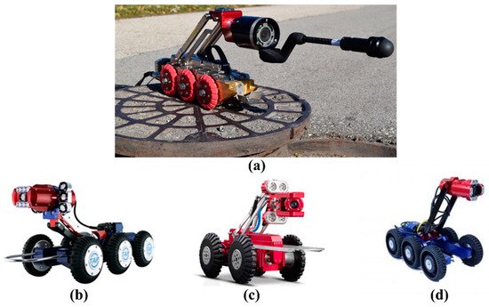
Currently, many data collection robotic systems have emerged that are capable of assisting workers with sewer inspection and spot repair. Table 1 lists the latest advanced robots along with their respective information, including the robot’s name, company, pipe diameter, camera feature, country, and main strong points. Figure 4 introduces several representative robots that are widely utilized to acquire images or videos from underground infrastructures. As shown in Figure 4a, LETS 6.0 is a versatile and powerful inspection system that can be quickly set up to operate in 150 mm or larger pipes. A representative work (Robocam 6) of the Korean company TAP Electronics is shown in Figure 4b. Robocam 6 is the best model to increase the inspection performance without the considerable cost of replacing the equipment. Figure 4c is the X5-HS robot that was developed in China, which is a typical robotic crawler with a high-definition camera. In Figure 4d, Robocam 3000, sold by Japan, is the only large-scale system that is specially devised for inspecting pipes ranging from 250 mm to 3000 mm. It used to be unrealistic to apply the crawler in huge pipelines in Korea.
|
Name |
Company |
Pipe Diameter |
Camera Feature |
Country |
Strong Point |
|---|---|---|---|---|---|
Description |
Ref. |
|
ID |
Number of Images |
Algorithm |
Task |
Performance |
Ref. |
|||||||
|---|---|---|---|---|---|---|---|---|---|---|---|---|
|
Accuracy (%) |
Processing Speed |
|||||||||||
|
CAM160 (https://goolnk.com/YrYQob accessed on 20 February 2022) |
Sewer Robotics |
200–500 mm |
||||||||||
|
1 | NA |
Broken, crack, deposit, fracture, hole, root, tap |
USA |
● Auto horizon adjustment ● Intensity adjustable LED lighting ● Multifunctional |
||||||||
NA |
NA |
4056 |
Canada |
[9] |
||||||||
|
Precision |
The proportion of positive samples in all positive prediction samples |
|||||||||||
|
1 |
3 classes | [9] |
||||||||||
Multiple binary CNNs |
Classification |
Accuracy: 86.2 Precision: 87.7 Recall: 90.6 |
NA |
LETS 6.0 (https://ariesindustries.com/products/ accessed on 20 February 2022) |
Recall |
The proportion of positive prediction samples in all positive samples |
[36] | |||||
|
2 |
ARIES INDUSTRIES |
150 mm or larger |
Self-leveling lateral camera or a Pan and tilt camera |
|||||||||
|
2 |
Connection, crack, debris, deposit, infiltration, material change, normal, root |
12 classes 1440 × 720–320 × 256 |
[48] |
|||||||||
Single CNN |
RedZone® Solo CCTV crawler |
Classification USA |
12,000 |
● Slim tractor profile ● Superior lateral camera ● Simultaneously acquire mainline and lateral videos |
||||||||
AUROC: 87.1 | AUPR: 6.8 | USA |
NA |
wolverine® 2.02 |
ARIES INDUSTRIES |
150–450 mm |
||||||
|
3 | NA |
Accuracy USA |
Attached deposit, defective connection, displaced joint, fissure, infiltration, ingress, intruding connection, porous, root, sealing, settled deposit, surface ● Powerful crawler to maneuver obstacles |
1040 × 1040 |
Front-facing and back-facing camera with a 185∘ wide lens ● Minimum set uptime |
The proportion of correct prediction in all prediction samples 2,202,582 ● Camera with lens cleaning technique |
||||||
|
3 |
Dataset 1: 2 classes | |||||||||||
Two-level hierarchical CNNs |
Classification |
Accuracy: 94.5 Precision: 96.84 Recall: 92 | The Netherlands |
F1-score: 94.36 [ |
1.109 h for 200 videos |
[38][ |
X5-HS (https://goolnk.com/Rym02W accessed on 20 February 2022) |
|||||
] |
4 |
EASY-SIGHT |
F1-score Dataset 1: defective, normal 300–3000 mm |
Harmonic mean of precision and recall |
NA |
[38 ≥2 million pixels |
China |
|||||
|
Dataset 2: 6 classes |
Accuracy: 94.96 Precision: 85.13 Recall: 84.61 | ][69] |
NA | ● High-definition |
40,000 ● Freely choose wireless and wired connection and control |
China | ● Display and save videos in real time |
|||||
[ | ] | [ | 69] |
Robocam 6 ( | ||||||||
F1-score: 84.86https://goolnk.com/43pdGA accessed on 20 February 2022) |
FAR TAP Electronics |
False alarm rate in all prediction samples |
||||||||||
|
8 classes |
600 mm or more |
Deep CNN Sony 130-megapixel Exmor 1/3-inch CMOS |
Korea |
Classification ● High-resolution ● All-in-one subtitle system |
||||||||
Accuracy: 64.8 | NA |
[ |
RoboCam Innovation4 |
TAP Electronics |
600 mm or more |
Sony 130-megapixel Exmor 1/3-inch CMOS |
Korea |
● Best digital record performance ● Super white LED lighting ● Cableless |
||||
|
Robocam 30004 |
TAP Electronics’ Japanese subsidiary |
250–3000 mm |
Sony 1.3-megapixel Exmor CMOS color |
Japan |
● Can be utilized in huge pipelines ● Optical 10X zoom performance |
|||||||
3.1.2. Benchmarked Dataset
Open-source sewer defect data is necessary for academia to promote fair comparisons in automatic multi-defect classification tasks. In this survey, a publicly available benchmark dataset called Sewer-ML [35][125] for vision-based defect classification is introduced. The Sewer-ML dataset, acquired from Danish companies, contains 1.3 million images labeled by sewer experts with rich experience. Figure 5 shows some sample images from the Sewer-ML dataset, and each image includes one or more classes of defects. The recorded text in the image was redacted using a Gaussian blur kernel to protect private information. Besides, the detailed information of the datasets used in recent papers is described in Table 2. This rpapesearchr summarizes 32 datasets from different countries in the world, of which the USA has 12 datasets, accounting for the largest proportion. The largest dataset contains 2,202,582 images, whereas the smallest dataset has only 32 images. Since the images were acquired by various types of equipment, the collected images have varied resolutions ranging from 64 × 64 to 4000 × 46,000.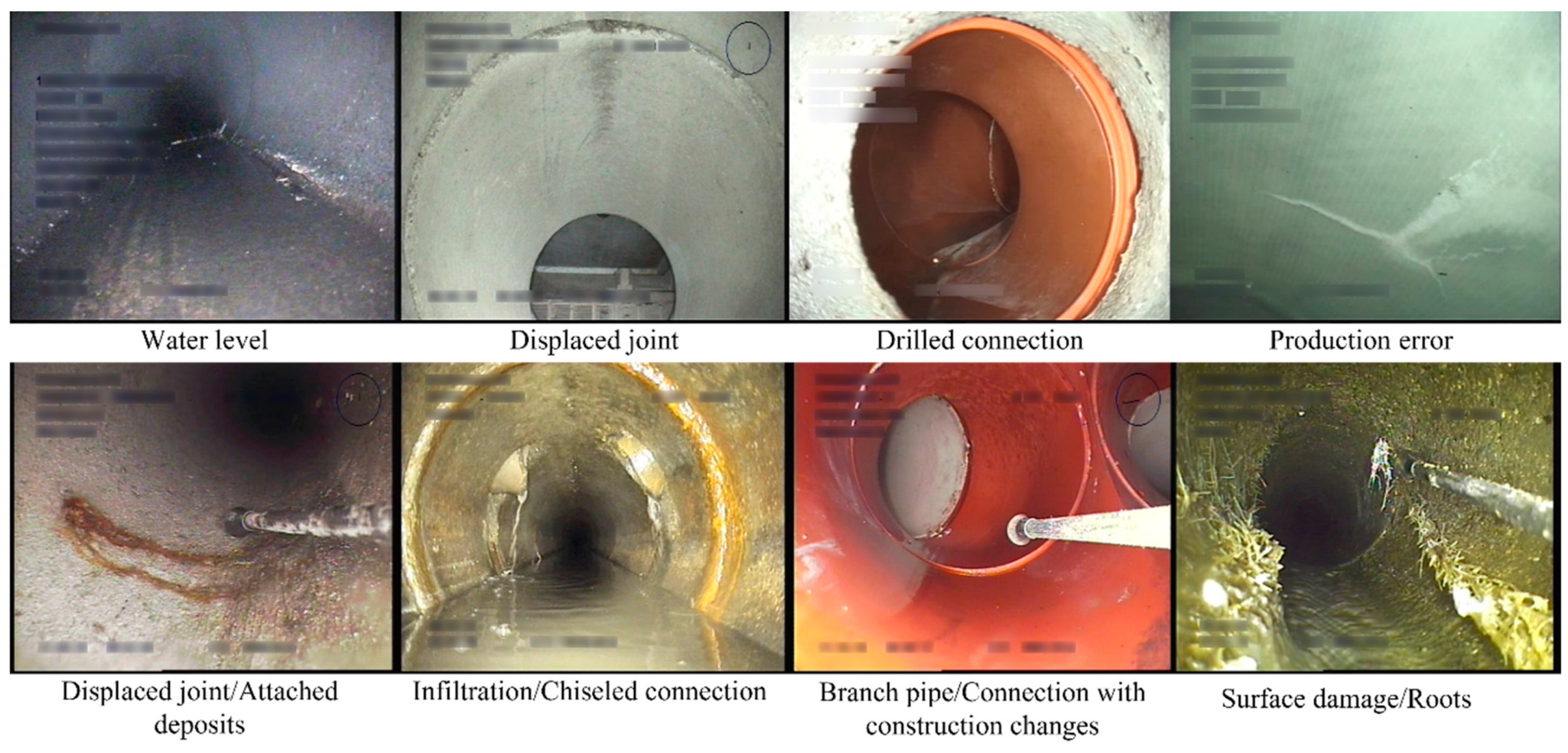

|
ID |
Defect Type |
Image Resolution |
Equipment |
Number of Images |
Country |
Ref. | ||||||||||
|---|---|---|---|---|---|---|---|---|---|---|---|---|---|---|---|---|
Dataset 2: barrier, deposit, disjunction, fracture, stagger, water | ||||||||||||||||
15,000 |
||||||||||||||||
] | [ | ] |
5 |
True accuracy Broken, deformation, deposit, other, joint offset, normal, obstacle, water |
||||||||||||
|
5 |
The proportion of all predictions excluding the missed defective images among the entire actual images |
1435 × 1054–296 × 166 |
[ NA |
18,333 |
] China |
|||||||||||
6 classes | [58] |
|||||||||||||||
CNN |
Classification |
Accuracy: 96.58 |
NA |
6 |
AUROC Attached deposits, collapse, deformation, displaced joint, infiltration, joint damage, settled deposit |
mAP | ||||||||||
|
4 | Area under the receiver operator characteristic (ROC) curve NA |
NA |
1045 |
[ China |
||||||||||||
|
6 | ][49] | [ | ||||||||||||||
8 classes |
CNN | ] |
Classification | [ |
Accuracy: 97.6 41] |
|||||||||||
0.15 s/image | [ | ][52] |
7 |
Circumferential crack, longitudinal crack, multiple crack |
AUPR |
Area under the precision-recall curve 320 × 240 |
NA |
335 |
[37 | |||||||
|
7 |
7 classes | ][49] |
Multi-class random forest |
Classification USA |
Accuracy: 71 |
25 FPS [11] |
||||||||||
[ | ] | [ | ] |
8 |
Debris, joint faulty, joint open, longitudinal, protruding, surface |
NA |
mAP first calculates the average precision values for different recall values for one class, and then takes the average of all classes |
|||||||||
|
8 | Robo Cam 6 with a 1/3-in. SONY Exmor CMOS camera |
48,274 |
[ South Korea |
9] [ |
||||||||||||
7 classes |
SVM | ] | [ | 71] |
||||||||||||
Classification | Accuracy: 84.1 |
NA |
9 |
Detection rate Broken, crack, debris, joint faulty, joint open, normal, protruding, surface |
The ratio of the number of the detected defects to total number of defects 1280 × 720 |
Robo Cam 6 with a megapixel Exmor CMOS sensor |
115,170 |
South Korea |
||||||||
|
9 | [ |
3 classes | ||||||||||||||
SVM |
Classification |
Recall: 90.3 Precision: 90.3 | ] | [ |
10 FPS52] |
|||||||||||
[ | ] |
10 |
Error rate Crack, deposit, else, infiltration, joint, root, surface |
NA |
Remote cameras |
|||||||||||
|
10 | 2424 | The ratio of the number of mistakenly detected defects to the number of non-defects |
3 classes UK |
|||||||||||||
CNN |
Classification |
Accuracy: 96.7 Precision: 99.8 Recall: 93.6 F1-score: 96.6 | [ | |||||||||||||
15 min 30 images | [ | ][73] |
11 |
Broken, crack, deposit, fracture, hole, root, tap |
PA NA |
|||||||||||
|
11 |
Pixel accuracy calculating the overall accuracy of all pixels in the image |
3 classes |
NA |
1451 |
Canada |
|||||||||||
RotBoost and statistical feature vector |
Classification |
Accuracy: 89.96 |
1.5 s/image |
12 |
Crack, deposit, infiltration, root |
1440 × 720–320 × 256 |
RedZone® Solo CCTV crawler |
3000 |
USA |
mPA |
||||||
|
12 |
The average of pixel accuracy for all categories |
] | ||||||||||||||
7 classes |
Neuro-fuzzy classifier |
Classification |
Accuracy: 91.36 | [ |
NA |
|||||||||||
[ | ] | [ | ] |
13 |
mIoU Connection, fracture, root |
The ratio of intersection and union between predictions and GTs |
4 classes 1507 × 720–720 × 576 |
Front facing CCTV cameras |
Multi-layer perceptions 3600 |
USA |
||||||
|
13 | Classification | Accuracy: 98.2 |
14 |
fwIoU Crack, deposit, root |
Frequency-weighted IoU measuring the mean IoU value weighing the pixel frequency of each class 928 × 576–352 × 256 |
NA |
3000 |
USA |
||||||||
NA | [ | ] |
||||||||||||||
|
14 |
2 classes |
Rule-based classifier |
Classification |
Accuracy: 87 FAR: 18 Recall: 89 |
NA |
15 |
||||||||||
|
15 |
Crack, deposit, root |
2 classes 512 × 256 |
OCSVM NA |
Classification1880 |
USA |
[ |
Accuracy: 75 |
|||||||||
NA | [ | ][65] |
16 |
Crack, infiltration, joint, protruding |
1073 × 749–296 × 237 |
NA |
||||||||||
|
16 | 1106 |
4 classes |
China |
CNN [49] |
Classification |
Recall: 88 Precision: 84 Accuracy: 85 [122] |
||||||||||
NA | [ | ][67] |
17 |
Crack, non-crack |
64 × 64 | |||||||||||
|
17 |
2 class |
Rule-based classifierNA |
40,810 |
Classification |
Accuracy: 84 FAR: 21 True accuracy: 95 Australia |
NA |
||||||||||
[ | ] | [ | 58] |
18 |
||||||||||||
|
18 |
Crack, normal, spalling |
4 classes 4000 × 46,000–3168 × 4752 |
RBN Canon EOS. Tripods and stabilizers |
Classification 294 |
Accuracy: 95 China |
NA |
19 |
Collapse, crack, root |
NA |
SSET system |
239 |
USA |
||||
|
20 |
Clean pipe, collapsed pipe, eroded joint, eroded lateral, misaligned joint, perfect joint, perfect lateral |
|||||||||||||||
|
19 |
7 classes |
YOLOv3 |
Detection |
mAP: 85.37 |
33 FPS |
[9]NA |
SSET system |
500 |
USA |
|||||||
|
20 |
4 classes |
Faster R-CNN |
Detection |
mAP: 83 |
9 FPS |
21 |
||||||||||
|
21 |
Cracks, joint, reduction, spalling |
3 classes 512 × 512 |
Faster R-CNN CCTV or Aqua Zoom camera |
Detection 1096 |
Canada |
[54] |
||||||||||
mAP: 77 | 110 ms/image |
22 |
||||||||||||||
|
22 |
Defective, normal |
3 classes NA |
Faster R-CNN CCTV (Fisheye) |
Detection 192 |
Precision: 88.99 Recall: 87.96 F1-score: 88.21 USA |
110 ms/image |
||||||||||
[ | ] | [ | ] |
23 |
Deposits, normal, root |
|||||||||||
|
23 |
2 classes |
1507 × 720–720 × 576 |
CNN Front-facing CCTV cameras |
3800 |
USA |
Detection |
Accuracy: 96 Precision: 90 |
0.2782 s/image |
||||||||
[ | ] | [ | ] |
24 |
Crack, non-crack |
|||||||||||
|
24 |
3 classes | 240 × 320 |
CCTV |
Faster R-CNN 200 |
South Korea |
|||||||||||
Detection | mAP: 71.8 |
110 ms/image |
25 |
Faulty, normal |
NA |
CCTV |
8000 |
|||||||||
|
SSD |
mAP: 69.5 |
57 ms/image | UK | |||||||||||||
|
26 |
Blur, deposition, intrusion, obstacle |
NA |
||||||||||||||
|
YOLOv3 | CCTV |
mAP: 53 12,000 |
33 ms/image NA |
|||||||||||||
|
27 |
Crack, deposit, displaced joint, ovality |
NA |
CCTV (Fisheye) |
|||||||||||||
|
25 |
2 classes |
Rule-based detector |
Detection |
32 |
Qatar |
[ |
Detection rate: 89.2 Error rate: 4.44 |
1 FPS |
||||||||
[ | ] | [ | ] |
29 |
Crack, non-crack |
320 × 240–20 × 20 |
||||||||||
|
26 |
2 classes |
GA and CNN |
CCTV |
Detection 100 |
NA |
|||||||||||
Detection rate: 92.3 | NA |
30 |
||||||||||||||
|
27 |
Barrier, deposition, distortion, fraction, inserted |
5 classes 600 × 480 |
SRPN CCTV and quick-view (QV) cameras |
Detection 10,000 |
China |
mAP: 50.8 Recall: 82.4 [ |
153 ms/image |
|||||||||
[ | ] | [ | ] |
31 |
Fracture |
|||||||||||
|
28 | NA |
CCTV |
1 class2100 |
USA |
CNN and YOLOv3 |
Detection |
AP: 71 |
65 ms/image |
||||||||
|
32 |
Broken, crack, fracture, joint open |
NA |
CCTV |
291 |
China |
3.2. Evaluation Metric
The studied performances are ambiguous and unreliable if there is no suitable metric. In order to present a comprehensive evaluation, multitudinous methods are proposed in recent studies. Detailed descriptions of different evaluation metrics are explained in Table 3. Table 4 presents the performances of the investigated algorithms on different datasets in terms of different metrics.|
Metric |
|---|
[ | ||||||
] | ||||||
[ | ||||||
] | ||||||
29 | ||||||
3 classes | ||||||
DilaSeg-CRF | ||||||
Segmentation | ||||||
PA: 98.69 | ||||||
mPA: 91.57 | ||||||
mIoU: 84.85 | fwIoU: 97.47 | 107 ms/image |
||||
|
30 |
4 classes |
PipeUNet |
Segmentation |
mIoU: 76.37 |
32 FPS |