Bayesian Nonlinear Mixed Effects Models: Comparison
Please note this is a comparison between Version 1 by Se Yoon Lee and Version 2 by Jason Zhu.

Nonlinear mixed effects models have become a standard platform for analysis when data is in the form of continuous and repeated measurements of subjects from a population of interest, while temporal profiles of subjects commonly follow a nonlinear tendency. While frequentist analysis of nonlinear mixed effects models has a long history, Bayesian analysis of the models has received comparatively little attention until the late 1980s, primarily due to the time-consuming nature of Bayesian computation. Since the early 1990s, Bayesian approaches for the models began to emerge to leverage rapid developments in computing power, and have recently received significant attention due to (1) superiority to quantify the uncertainty of parameter estimation; (2) utility to incorporate prior knowledge into the models; and (3) flexibility to match exactly the increasing complexity of scientific research arising from diverse industrial and academic fields. 

  • Bayesian Nonlinear Mixed Effects Models

1. Introduction

One of the common challenges in biological, agricultural, environmental, epidemiological, financial, and medical applications is to make inferences on characteristics underlying profiles of continuous, repeated measures data from multiple individuals within a population of interest [1][2][3][4][1,2,3,4]. By  ‘repeated measures data’ researcherswe mean the data type generated by observing a number of individuals repeatedly under differing experimental conditions, where the individuals are assumed to constitute a random sample from a population of interest. A  common type of repeated measures data is longitudinal data such that the observations are ordered by time [5][6] [5,6].
Linear mixed effects models for repeated measures data have become popular due to their straightforward interpretations, flexibility allowing correlation structure among the observations, and utility accommodating unbalanced and multi-level data structure (i.e., clustered designs that vary among individuals) [7][8][7,8]. The modeling framework is also intuitively appealing: the central idea that individuals’ responses are governed by a linear model with slope or intercept parameters that vary among individuals seems to be appropriate in many scientific problems (for, e.g., see  [9][10][9,10]). It also allows practitioners to test and evaluate multivariate causal relationships by conducting regression analysis at the population level. By preserving the multi-level structure in a single model, estimation or prediction for the analyses can take advantage of information borrowing [11].
For many applications, researchers often want to theorize that time courses of individual response commonly follow a certain nonlinear function dictated by a finite number of parameters [12]. These nonlinear functions are based on reasonable scientific hypotheses, typically represented as a differential equation system. By tuning the parameters, the shape of the function in terms of curvature, steepness, scale, height, etc., may change, which is used as the rationale behind describing heterogeneity between subjects. Nonlinear mixed effects models, also referred to as hierarchical nonlinear models, have gained broad acceptance as a suitable framework for these purposes [13][14][15][13,14,15]. Analyses based on this model are now routinely reported in various industrial problems, which is, in part, enabled by the breakthrough development of software [16][17][18][19][20][16,17,18,19,20]. The excellent books and review papers were published by  [14][15][21][14,15,21]. Although their works were published more than 20 years ago, they still provide statisticians, programmers, and researchers with many pedagogical insights about the modeling framework, implementations, and practical applications of using the nonlinear mixed effects models.
While frequentist analysis of nonlinear mixed effects models has a long history, Bayesian analysis for the models was a relatively dormant field until the late 1980s. This is due primarily to the time-consuming nature of the calculations required for Bayesian computation to implement a Bayesian model [22]. Since the early 1990s, Bayesian approaches began to re-emerge, motivated both by exploitation of rapid developments in computing power and by the growing desire to quantify the uncertainty associated with parameter estimation and prediction [23][24][25][23,24,25]. Since then, Bayesian nonlinear mixed effects models, also called Bayesian hierarchical nonlinear models, have been extensively used in diverse industrial and academic researches, endowed with new computational tools providing a far more flexible framework for statistical inference exactly matching the increasing complexity of scientific research [26][27][28][29][30][31][26,27,28,29,30,31].

2. Trends and Workflow of Bayesian Nonlinear Mixed Effects Models

2.1. Rise in the Use of Bayesian Approaches for the Nonlinear Mixed Effects Models

As of January 1970 to December 2021, PubMed.gov (https://pubmed.ncbi.nlm.nih.gov/, accessed on 23 February 2022) searched of “nonlinear mixed-effect models” yielded 6288 publications. Among the published articles, nearly 94% of works used frequentist approaches (5929 articles), while only 6% of works adopted Bayesian approaches (359 articles). 
The dormancy of the Bayesian approaches until the late 1980s is mainly due to the time-consuming nature of the calculations based on a sampling scheme, which was previously impossible by the limitation of computing power. Fortunately, a breakthrough in computer processors (for, e.g., Am386 in 1991, Pentium Processor in 1993, etc.) took place in the early 1990s, driving the computing revolution to solve computationally intense problems, and this has given the statistical community the ability to solve statistical questions by using Bayesian methods. This timeline is also aligned with the widespread Markov chain Monte Carlo (MCMC) sampling techniques in the Bayesian community [32][33][32,33]. Since then, the Bayesian community has been gradually gaining the momentum to leverage the rapidly growing developments of computing power, and now, assorted Bayesian software packages (e.g., JAGS [34], BUGS [35], and Stan [17]) are available for researchers to answer scientific questions arising from industrial and academic research.
To understand the rise of the Bayesian approaches, we it should be first want to understanded what will be some of the advantages of using Bayesian methods over frequentist methods in the context of nonlinear mixed effects models. As  the primary focus is of this review paper is to provide the readers with some insight on methodologies and practical implementation of using Bayesian approaches, theour comparison and exposition below are described from an operational viewpoint. 
The stark difference between using frequentist and Bayesian approaches may be the procedure of describing an uncertainty underlying the parameter estimation for the nonlinear mixed effects models. Here, the parameter which is of primary interest is the population-level parameters (also called fixed effects), typical values for the individual-level parameters. In many cases, frequentist 95%
confidence intervals for the parameters of the models are constructed by assuming that asymptotic normality of maximum likelihood estimator holds in a finite sample study, which is actually the most accurate in large sample scenario [36][51]. Most frequentist software packages, such as NONMEM [13][37][13,47], Monolix [38][48], and nlmixr [18], by default, may print out a 95% confidence interval of the form, “Estimate ± 1.96 × Standard Error”, or some transformation of the lower and upper bounds, if necessary, such that the Standard Error is calculated by using (observed) Fisher information matrix [39][40][41][52,53,54]. Using such a scheme in small sample studies is highly likely to overlook the gap between the reality of the data and the idealistic asymptotic situation.
In contrast, as for the Bayesian approaches, the large-sample theory is not needed for the uncertainty quantification, and the procedure to obtain 95% posterior credible intervals is a lot easier than obtaining 95% confidence intervals (See Chapter 4 of [42][55]). Furthermore, Bayesian credible intervals based on percentiles of posterior samples allow for a strongly skewed distribution, wherein frequentist confidence intervals (based on large-sample theory) may induce a non-negligible approximating error due to the deviation from the asymptotic normality. Along with that, Bayesian methods are highly appreciated when researchers wish to incorporate prior knowledge from previous studies into the model so that posterior inference provides the researchers with an updated view on the problem, possibly with a more accurate estimation. Using prior information would be particularly useful in small-sample contexts [43][44][56,57]. For example, in medical device clinical trials, some opportunities and challenges in developing a new medical device are: (i) there is often a great deal of prior information for a medical device; (ii) a medical device evolves in relatively small increments from previous generations to a new generation; (iii) there are only a few numbers of patients for the trials; and (iv) companies need to make a rational decision promptly to reduce cost. In those settings, Bayesian methods have been demonstrated to be suitable, and their proper use is guided by Food and Drug Administration [45][46][58,59].

2.2. Bayesian Workflow

RWesearchers outline the first two steps in the Bayesian workflow of using Bayesian nonlinear mixed effect models described in Figure 1. The  panel includes some mathematical notations that are consistently used throughout the paper. These notations will be clearly understood later. The  aim of our explanation at this point is to provide readers with a blueprinted plan to implement Bayesian modeling strategies for the nonlinear mixed effects models. ResearchersWe assume that readers are familiar with basic concepts and generic workflow in Bayesian statistics; see [55,60,61] [42][47][48] for those basic concepts and refer to the review paper by [49][62] and references therein for detailed concepts and general terminologies used in workflow, such as prior and posterior predictive checks, and prior elicitation, etc.
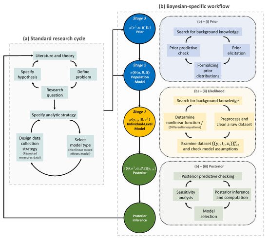
Figure 1. The Bayesian research cycle. A research cycle using Bayesian nonlinear mixed effects model comprises two steps: (a) standard research cycle and (b) Bayesian-specific workflow. Standard research cycle involves literature review, defining a problem and specifying the research question and hypothesis. Bayesian-specific workflow comprises three sub-steps: (b)–(i) formalizing prior distributions based on background knowledge and prior elicitation; (b)–(ii) determining the likelihood function based on a nonlinear function f; and (b)–(iii) making a posterior inference.
The first step of the Bayesian research cycle is (a) standard research cycle [50][51][63,64]. Some early activities at this step involve reviewing literature, defining a problem, and specifying a research question and a hypothesis. After that, researchers specify which analytic strategy would be taken to solve the research question and suggest possible model types, followed by data collection. The data type arising in this process may include a response variable and some covariates that are grouped longitudinally, which then formulates repeated measures data of a population of interest. Furthermore, if there appears to be some nonlinear temporal tendency at each subject, then a possible model type for the analysis is a nonlinear mixed effects model [15][52][15,65]. The second step of the Bayesian research cycle is (b) Bayesian-specific workflow. Logically, the first thing to do at this step is to determine prior distributions (see Step (b)–(i) in Figure 1). The selection of priors is often viewed as one of the most crucial choices that a researcher makes when implementing a Bayesian model, as it can have a substantial impact on the final results [53][66]. As exemplified earlier in the context of Bayesian medical device trials, using a prior in small sample studies may improve the estimation accuracy, but an unthoughtful choice of priors would lead to a significant bias in estimation. Prior elicitation effort would require Bayesian expertise to formulate domain expert’s knowledge in a probabilistic form [54][67]. Strategies for prior elicitation include asking domain experts to provide suitable values for the hyperparameters of the prior [55][56][68,69]. After prior is specified, one can check the appropriateness of the priors through prior predictive checking process [57][70]. For almost all practical problems, prior distribution of Bayesian nonlinear mixed effect models can be hierarchically represented as follow: (1) a prior for the parameters used in likelihood, often called ‘population-level model’ in the literature of mixed effects modeling; and (2) a prior for the parameters used in the population-level model and for the parameters describing the residual errors used in likelihood. It is important to note that the former type of prior distribution (that is, (1)) is also a requirement to implement frequentist approaches for the nonlinear mixed effects model, as a name of ‘distribution for random effects’. The second task is to determine the likelihood function (see Step (b)–(ii) in the panel). At  this time, the  raw dataset collected in (a) standard research cycle should be cleaned and preprocessed. Before  embarking on more serious statistical modeling, it is a common practice to get some insight about the research question via exploratory data analysis and have a discussion with domain experts such as clinical pharmacologists, clinicians, physicians, engineers, etc. To  some extent, eventually, all these efforts are to determine a nonlinear function (denoted as f in this paper) that best describes the temporal profiles of all subjects. This nonlinear function is a known function because it should be specified by researchers. In other words, the branch of the nonlinear mixed effects models belongs to parametric statistics. However, one technical challenge is that, in many problems, such a nonlinear function is represented as a solution of a differential equation system [58][59][71,72], and  therefore there is no guarantee that peoplewe can conveniently work with a closed-form expression of the nonlinear function. For  example, if  researchers wish to work with nonlinear differential equations [60][61] [73,74], then some approximation via differential equation solver [62][63][75,76] may be needed to calculate the nonlinear function. As such, most software packages dedicated to implementing a nonlinear mixed effect model, or, more generally, a Bayesian hierarchical model, are equipped with several built-in differential equation solvers [17][37][64][17,47,77]. For instance, visit the website (https://mc-stan.org/docs/2_29/stan-users-guide/ode-solver.html, accessed on 20 February 2022) to see some functionality supported in Stan [17]. Finally, the likelihood is combined with the prior to form the posterior distribution (see Step (b)–(iii) in the panel). Given the important roles that the prior and the likelihood have in determining the posterior, this step must be conducted with care. The implementational challenge at this step is to construct an efficient MCMC sampling algorithm. The basic idea behind MCMC here is the construction of a sampler that simulates a Markov chain that is converging to the posterior distribution. One can use software packages if prior distributions to be implemented in Bayesian models exist in the list of prior options available in the packages. Otherwise, professional programmers and Bayesian statisticians are needed to make codes manually; this review paper will be useful for that purpose.