Your browser does not fully support modern features. Please upgrade for a smoother experience.
Please note this is a comparison between Version 2 by Dean Liu and Version 1 by Matthew Richard Tarasek.
Multi-parametric magnetic resonance imaging (MRI) is a paradigm that combines several MR imaging contrast types to provide added layers of information for the characterization of tissue types, including benign and malignant tumors.
- tissue characterization
- MRI
- thermal sensitivity
- in vivo
1. Introduction
The clinical applications of magnetic resonance (MR) imaging in oncology are rapidly evolving from subjective and interpretive diagnostic tests based on tissue morphology to more quantitative approaches that probe tissue biology. The best possible characterization of cancer in MR imaging is currently achieved by a multi-parametric approach that supplements conventional MRI with additional functional MRI techniques [1,2,3,4]. These techniques provide added layers of information on features such as tumor metabolism, cellular microenvironment, and tumor vascularity [2,4,5,6,7]. Despite ongoing research into multi-parametric MRI [8,9,10,11], there are still limitations in detecting and delineating early-stage cancer lesions when they are curable [4]. MR imaging provides the best spatial resolution and anatomical soft tissue contrast, but there is still a need to develop novel MR imaging approaches to improve tissue characterization, reduce unwanted biopsies, and provide additional information to guide cancer therapy treatments. The lack of multi-parametric MR datasets is a major clinical impediment in cancer screening and therapy planning, even in the most common cancer types.
2. MR Imaging Experiments with Temperature Modulation
MR thermometry and temperature probe data were used to ensure that steady-state temperatures were achieved before quantitative parameter measurements were acquired. Figure 31a, b depicts warming data plots with MRT and temperature probe data for tumor tissue (blue oval ROIs) and surrounding muscle tissues (red rectangle ROIs). Muscle ROIs were selected to minimize fat content. The oil vials seen in the axial images were used for B0 drift correction in the PRFS measurements. External oil phantoms were also used to verify reproducibility in T1/T2 measurement at high and low temperatures [28]. All oil T1/T2 measurements were within 2.5% during the 2-h scan sessions. Similar plots to Figure 31b were observed for all rats imaged and provide a confirmation of temperature change and stabilization for quantitative imaging. MRT measurements were always within 1 °C of fiber optic probe measurements. All rats were heated from an initial temperature of 26 °C as discussed in the Materials and Methods section.
Figure 31. In vivo MR thermometry data and temperature probe data. (a) Axial slice through the center of a tumor grown on a rat flank. The elliptical ROI averages the MRT data in the tumor region, while the rectangular ROIs average MRT data in the muscle region. (b) Temperature change plots during warming cycle for muscle (diamond markers) and tumor (round markers) tissues. Plot also indicates rectal (body) and tumor temperature probe readings at various timepoints.
For all tumor models analyzed ian this work, we d researchers found a statistically significant difference (p < 0.05) between one or more delta-quantitative contrast measurements (%ΔΓ/°C) for all tumor/muscle pairs. Figure 42a–d presents an example of low-temperature and high-temperature quantitative image parameter maps for reconstructed T1, T2, and ADC images of a MAT B III tumor. Here, MRI data were fitted per pixel to obtain the quantitative maps. In all experiments the rat required some repositioning to check temperature probe placements. An example of this repositioning can be seen when comparing positional differences in Figure 42 top and bottom. Overall, the slices selected for the imaging volume were very similar as this was determined by the center mass of the xenograft tumor in localizer scans. Unfortunately, due to movement a direct mapping of parameter change could not be achieved. Table 1 shows the fit quantities (mean and standard deviation) for each tumor/muscle contrast type, and their respective %ΔΓ/°C. Most notably, we researchers found significant difference in %ΔT1/°C and %ΔADC/°C for MAT B III tumor compared to its surrounding muscle, along with a significant difference in %ΔT2/°C and %ΔADC/°C for MatLyLuB2 compared to its surrounding muscle tissue. Blue bolded values in Table 1 indicate the statistically significant differences for all measured %Δ°C (t-test result p-value < 0.05). Box plots of highlighted values from Table 1 are presented in Figure 53. Each point plotted here represents four measurements for each tumor type or its surrounding muscle tissue.
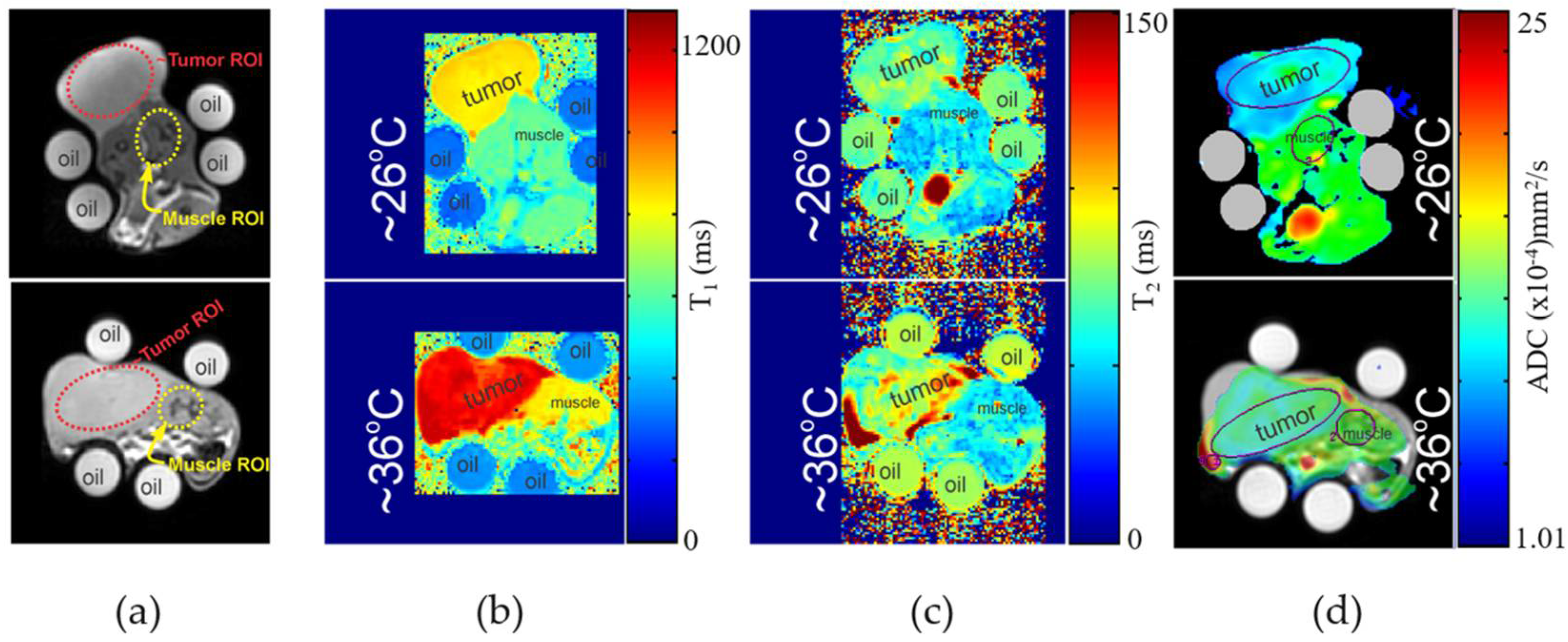
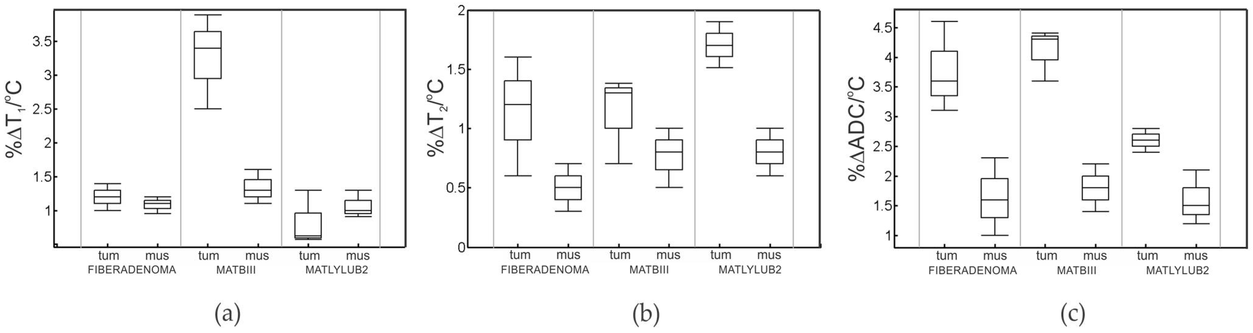
Figure 42. (a) Reference axial images of the same rat (top and bottom) with MAT B III tumor. Top images in (b–d) are quantitative T1, T2, and ADC maps, respectively, at 26 °C. Bottom images in (b–d) are quantitative T1, T2, and ADC maps, respectively, at 36 °C. General locations of the tumor and muscle regions are indicated on the images.
Figure 53. Box plots of MR thermal contrast change with temperature: (a) %ΔT1/°C, (b) %ΔT2/°C, and (c) %ΔADC/°C. Columns represent benign breast, malignant breast (MAT B III), and malignant prostate (MatLyLuB2), respectively (labeled “tum”), and muscle regions that were selected near those respective tumors (labelled “mus”). Each point plotted here represents 4 measurements for each tumor type or its surrounding muscle tissue.
Table 1. Summary of (i) quantitative quantities a and (ii) thermally-induced changes in quantitative quantities b. Bolded quantities indicate t-test p-value < 0.05 for comparisons indicated in text.
| Fibroadenoma (Benign) | Breast Tumor/MAT B III | Prostate Tumor/ MatLyLuB2 |
||||
|---|---|---|---|---|---|---|
| Muscle c | Benign Tumor |
MuBreascle ct Malignant |
BrMuscleast Malignant c |
MuProscltate c Malignant |
Prostate Malignant |
|
| T1 (ms) a | 769 ± 12 | 651 ± 20 | 7671201 ± 1026 | 127701 ± 26 ± 13 | 7701145 ± 1322 | 1145 ± 22 |
| %ΔT1/°C b | 1.16 ± 0.20 | 1.20 ± 0.91 | 1.40 ± 0.423.41 ± 0.64 | 3.41 ± 0.641.05 ± 0.3 | 10.05 ± 0.360 ± 0.51 | 0.60 ± 0.51 |
| T2 (ms) a | 26.0 ± 0.75 | 23.8 ± 1.2 | 2563.8 ± 0.87 ± 2.1 | 263.7 ± 2.1.6 ± 0.6 | 26.6 ± 0.64.6 ± 1.7 | 64.6 ± 1.7 |
| %ΔT2/°C b | 0.50 ± 0.3 | 1.17 ± 0.8 | 01.72 ± 0.511 ± 0.7 | 10.11 ± 0.770 ± 0.3 | 0.70 ± 0.31.7 ± 0.9 | 1.7 ± 0.9 |
| ADC (×10−4 mm2/s) a | 14.88 ± 1.1 | 11.22 ± 1.6 | 148.91 ± 1.0 ± 1.7 | 813.9 ± 1.752 ± 1.2 | 10.3.52 ± 1.2 ± 1.4 | 10.3 ± 1.4 |
| %ΔADC/°C b | 1.6 ± 0.7 | 4.00 ± 0.78 | 1.8 ± 0.64.20 ± 0.81 | 4.20 ± 0.811.5 ± 0.6 | 1.5 ± 0.62.60 ± 0.56 | 2.60 ± 0.56 |
a Measurements were made at ~36 °C. Error reported from the calculated measurement stdev, b Measurements calculated as percent increase per degree Celsius. Absolute error reported from the propagation of 90% confidence intervals calculated as Ᾱ ± (ts/√n) where Ᾱ is the mean measured value, t is Student’s t, s is the measured stdev, and n is the number of measurements, c Muscle ROIs were selected near the corresponding benign or malignant tumors.
3. Tumor Histopathology
Histopathology provided a ground truth reference to determine a true positive result for malignant or benign tissue. A histopathology report of each tumor used in experiments was made to determine the general tissue morphology of the tumors as described in section II.A. H&E staining of the MAT B III and MatLyLuB2 tumors indicates that these tumors are indeed malignant breast and prostate carcinoma, respectively. When evaluating the H&E staining of the spontaneous mammary tumors, all were classified as benign fibroadenomas.