Probabilistic Optimization Techniques in Smart Power System

Probabilistic Optimization Techniques in Smart Power System: Comparison

Please note this is a comparison between Version 2 by Conner Chen and Version 1 by Sadiq Ahmad.

Stochastic programming is used to solve optimization problems in which the majority of the parameters are probabilistic. Probabilistic optimization can make efficient use of information, both in terms of selecting evaluation points and the message they convey. It can handle many sorts of noise and adapts to various aspects of optimization issues. Unlike deterministic optimization, probabilistic optimization techniques discover the best solution for data with randomness.

probabilistic optimization

1. Probabilistic Optimization

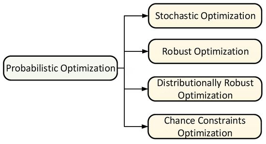
Stochastic programming is used to solve optimization problems in which the majority of the parameters are probabilistic [32]. Probabilistic optimization can make efficient use of information, both in terms of selecting evaluation points and the message they convey. It can handle many sorts of noise and adapts to various aspects of optimization issues. Unlike deterministic optimization, probabilistic optimization techniques discover the best solution for data with randomness [33]. As indicated in Figure 1, there are multiple probabilistic optimization categories: stochastic optimization, robust optimization, distributionally robust optimization, and chance-constrained optimization.

Figure 1.

Classification of probabilistic optimization.

1.1. Stochastic Optimization

Stochastic optimization is critical for addressing uncertainty in optimization problems. Due to computing problems, uncertainty is typically disregarded in classical optimization, but breakthroughs in computational techniques now allow for the efficient handling of uncertainties [34]. Stochastic optimization is concerned with strategies for minimising or optimising an uncertain objective function. In contrast to deterministic optimization issues, stochastic optimization problems do not have a single solution. To solve the issue tractably, structural assumptions such as a constraint on the size of the choice variables, the result space, or convexity are required [35]. Traditionally, stochastic optimization modeled uncertainties as random variables with well-defined distributions [36].

1.1.1. Architecture of Stochastic Optimization

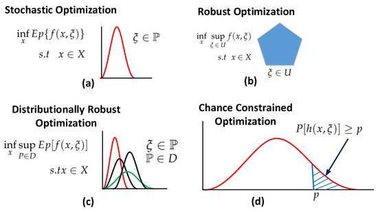
The objective function is typically optimized over the expected value of the uncertain parameters for the formulation of stochastic programming, as shown in Equation (1). Where x is the decision variable that belongs to set X,

E_{p}

is the expected value of the random variable

ξ

. Stochastic optimization is graphically represented in part a of Figure 2, where P is the probability distribution of random variable

ξ

. An exact distribution is required for the uncertainties, which cannot be estimated with the empirical data accurately [37]. Either all scenarios or scenarios with probability guarantees are feasible for the modeled solution. In stochastic optimization, sample-based techniques are commonly utilizeddue to the difficulty of obtaining the correct distribution of random variables. A greater sample size is utilizedto get higher probability guarantees, increasing computing complexity [34].

\begin{matrix} inf_{x} E p {f (x, ξ)} \\ s . t x \in X \end{matrix}

(1)

Figure 2. Graphical comparison of: (a) stochastic optimization; (b) robust optimization; (c) distributionally robust optimization; (d) chance constrained optimization.

The probability distribution determines the level of uncertainty in stochastic optimization. In basic scenarios, uncertainty is well known, but in practise, it is only partially unknown. The accuracy of stochastic optimization is influenced by the model specifics and availability of possible scenarios. If a stochastic framework is used for all scenarios, the problem becomes more difficult. A trade-off between number of scenarios and, computing time, and complexity is required [34].

1.1.2. Taxonomy of Stochastic Optimization

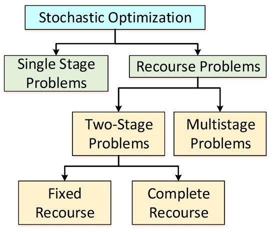
Stochastic optimization can be categorized into single stage problems and recourse problems. The recourse problems can be further classified into two stage and multistage problems as shown Figure 3 [25]. In single stage problems, a single but optimal decision is obtained where in recourse optimization problems, it is essential to know the probability distribution of the random variable in the first step, where the second step (correction of that decision) is being performed. In the two stage stochastic optimization the decision maker must make judgments in two stages (at two distinct times) for a given phenomenon with uncertainty. The first stage choice is critical since it must be made based on some random factors gleaned from previous experience or a survey.

Figure 3.

Taxonomy of stochastic optimization.

Two-stage stochastic optimization problems may have fixed recourse or complete recourse. In case of fixed recourse, the first stage is prediction stage where in second-stage, fixed decision is done based on the results of the experiment [38]. Two-stage stochastic optimization problems will be considered as a complete recourse if, for every scenario, there always exists a viable second solution [33]. Multistage stochastic programming is an extension of two stage stochastic programming to the sequential realization of uncertainty. Majority of the real time problems lies in the domain of multistage stochastic optimization which entail a series of decisions in response to changing outcomes over time [35].

1.2. Robust Optimization

Robust optimization is a relatively new technique for optimising in the presence of uncertainty. Rather than using a stochastic model, it uses a deterministic, set-based uncertainty model. The robust optimization solution is valid for any specification of the uncertainty in a given set. The reason for robust optimization is that it accounts for both set-based uncertainty and computational tractability [28]. Robust optimization and the respective computational tools deal with optimization problems in which the information are indeterminate and belong to some set of uncertainty [39]. Robust optimization ensures that the worst-case scenario is realized, ensuring that the solution is both practical and optimal for a given set of uncertainties. Robust optimization is not chosen in some applications due to its conservative nature, however it is used in the power industry to preserve reliability. Robust optimization necessitates a considerable amount of knowledge about the uncertainty, such as its size and range [34].

1.2.1. Architecture of Robust Optimization

Robust optimization is a realization of worst-case parameters that belong to the uncertainty set. Worst case realization of robust optimization sometimes becomes unrealistic in practice [37]. The architecture of robust optimization is available in Equation (2), where x is the decision variable that belongs to set X,

ξ

is a random variable belonging to the uncertainty set U. Robust optimization can be graphically represented as shown in part b of Figure 2.

\begin{matrix} inf_{x} sup_{ξ \in U munder f (x, ξ)} \\ s . t x \in X \end{matrix}

(2)

1.2.2. Taxonomy of Robust Optimization

Robust optimization can be categorized as shown in Figure 4, and is discussed as follows.

Figure 4.

Taxonomy of robust optimization.

Strict robustness: This optimization type is sometimes known as classic robust optimization, min–max optimization, absolute deviation, one-stage robustness, or simply robust optimization. It is treated, as the fundamental starting point in the area of robustness. A solution x is called strictly robust if it is feasible for all possible scenarios of uncertainty set U [40].
Cardinality constrained Robustness: In cardinality constrained robustness, reduction in uncertainty’s space can relax strictness in robust optimization. Analyzing the worst-case scenario in robust optimization, it is improbable that all the uncertainty set parameters will change simultaneously. Hence, it restricts uncertainty space by varying some parameters while considering fixed values for the remaining [41].
Adjustable robustness: In adjustable robustness, the uncertainty space of strict robustness gets relaxed by dividing uncertainty space into groups of variables such as here and now and wait-and-see. Variables from the here and now group must be evaluated before the scenario $ξ \in U$ is determined where variables from the wait-and-see group can be determined once the scenario $ξ$ is known [42].
Light robustness:In light robustness, relaxing the constraints in terms of quality can reduce the strictness of the robust optimization, rather than reducing the space of uncertainty. Light robustness develops a trade-off between quality and robustness of the solution [43].
Regret robustness: In regret robustness, the objective function relaxes the problem. Rather than to minimize the worst case performance of the solution, regret robustness reduces the difference of objective function having the best solution and the objective function that would have been possible in a scenario [44].
Recoverable robustness: Concept of recovery algorithm gets exploited in recoverable robustness and family of recovery algorithms which is represented by B. It provides the solution in two stages, such as adjustable robustness. A solution x is called recovery robust with respect to recovery algorithm A if for any probable situation $ξ \in U$ an algorithm $A \in B$ exist such that when A is applied to the solution x and the scenario $ξ$ makes a solution $A (x; ξ) \in F (ξ)$ [45].

1.3. Distributionally Robust Optimization

Distributionally robust optimization, also known as min–max stochastic programming, reduces the computational complexity of stochastic programming and conservative nature of robust optimization. It turns up optimal decisions for the worst-case probability distributions within a family of possible distributions, defined by specific characteristics such as their support vector and moments information [36]. As compare to stochastic programming, it is less dependent on the data having an exact probability distribution. Due to the incorporation of probability distribution and concept of ambiguity sets, the result becomes less conservative as compared to simple robust optimization [46].

1.3.1. Architecture of Distributionally Robust Optimization

A distributionally robust optimization or min–max stochastic programming model act as a bridge between robust and stochastic optimization. It usually takes the form, as shown in Equation (3). where x is the decision variable that belongs to set X, P is the probability distributions that belongs to an ambiguity set D,

ξ

is the random variable, and

E p

is expected value of the random variable [37]. Distributionally robust optimization can be graphically represented as shown in part c of Figure 2. The random variable

ξ

belongs to probability distribution P where P itself belongs to ambiguity set D.

(3)

1.3.2. Taxonomy of Distributionally Robust Optimization

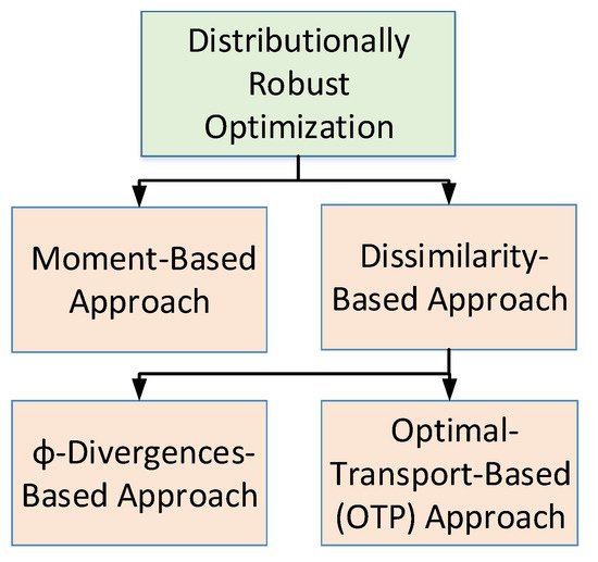
Various categories of distributionally robust optimization (DRO) are shown in Figure 5 and are discussed as follows. DRO is a strong modeling paradigm for optimization under uncertainty that arises from the realization that the probability distribution of uncertain parameters of the the problem is uncertain in-itself. As a result the concept of ambiguity set arises which is defined as a set in which the modeler considers that the real distribution of the uncertain parameters of problem has uncertainty. Naturally, the ambiguity set’s creation is critical to DRO’s actual effectiveness. DRO can be classified on the basis of characteristics and specifications of ambiguity set which are described as follows [47].

Figure 5.

Taxonomy of distributionally robust optimization.

(1): Moment-based approach: The ambiguity set in moment based approach is the set of all probability distributions whose moments satisfy certain constraints [

(1) Moment-based approach: The ambiguity set in moment based approach is the set of all probability distributions whose moments satisfy certain constraints [

49].
(2): Dissimilarity-based approach: The ambiguity set in this case is the set of all probability distributions whose dissimilarity to a nominal distribution is lower than or equal to a given value. In this category, the choice of the dissimilarity function leads to couple of different variants which are as follows [

(2) Dissimilarity-based approach: The ambiguity set in this case is the set of all probability distributions whose dissimilarity to a nominal distribution is lower than or equal to a given value. In this category, the choice of the dissimilarity function leads to couple of different variants which are as follows [

47].

(a)

Optimal-transport-based (OTP) approach: The authors in [50,51] applied Wasserstein distance as a dissimilarity function which shows some nice statistical convergence properties.

(b)

ϕ

-Divergences based approach: This group consist of all those techniques which uses

ϕ

-divergences such as Kullback–Leibler divergence, as was described in [52,53]. Approaches used in [54,55] are based on likelihood which also belongs to this category.

65].

The stochastic optimization method is used to solve a unit commitment problem with a demand response that is uncertain. It is demonstrated that by taking the uncertainty of demand response into account in a probabilistic manner, generating capacity may be enhanced [66]. The model was created to deal with uncertainty in the unit commitment problem while minimizing the system’s operating costs. To acquire an efficient solution for the system, parallelization and decomposition strategies are applied [67]. The integration of storage devices and a high penetration of renewable energy resources is demonstrated in a unit commitment and economic dispatch model. It is concluded that the consideration of storage devices to reduce operational cost is quite effective. Linear programming is used to formulate optimization problem in [66,67], where in [24] mixed-integer linear programming is applied.

For day-ahead optimal power flow, stochastic optimization is used, which can help to improve economic benefits. The uncertainties of wind power and load are incorporated into DC optimal power flow. The problem is expressed as a mixed integer linear programming problem that is solved using the two-point estimation approach. To determine the ideal number of switching each hour, a framework based on probability decisions is designed, taking into account risk cost and economic rewards [68].

2.2. Applications, Objectives and Solution Algorithms of Robust Optimization

In a smart power system, robust optimization has a variety of applications with dynamic objectives. Table 3 shows the applications, and Table 4 summarizes the objectives.

Table 3.

Applications of robust optimization and its problem Type.

Ref.	Applications	LP	NLP	MIP	MILP	MINLP	MIBLP	MISOCP	MIQP	QP
DD and IGDT	MPC and FPIM	BB	LM	QP	MCS	LOM and BMLM	IM
[69]
[92	SGEM	,			106,107		×					]	Minimize Generation Cost
	×			×										[70,71,72,73,75]	MEM			×
[	×	89,91		]	×
Minimize Electricity Cost		×		×											[90,91]	HEM
[76		×					]	Minimize Social Benefits Cost
						×						×		[88,89,93]	DSM		×	×		×
[73,77]	Minimize Microgrid Net Cost								×			×				[92,94]	PEV		×		×
[90]	Minimize Comfort Violation										×	,66]
				[67,78,83,	UC	84,85,87,95,	×	96,97,98,99,104]	UC		100,101	×	,102,
103,	×	×	×	×		×		×		[60]	STG				×
[65]	RDG				×

The energy management problem of a smart thermal grid with aquifer thermal energy storage is solved using a stochastic model predictive control framework. Mixed-integer quadratic programming is used to solve the problem. The developed model is used to capture the aquifer’s injection and extraction imbalances, as well as the undesired mutual interaction of aquifer thermal energy storage and smart thermal grid [60]. The problem of probabilistic optimal power dispatch for microgrid is defined as non-linear programming. The operating cost is minimizedthrough particle swarm optimization, and the optimization problem is handled appropriately [61].

In day-ahead transmission network planning, a probabilistic model is utilizedto schedule demand response. For the best demand response scheduling, network security and consumer economic factors are applied. Thermal units and renewable energy resources have been modeled, and the problem has been formulated using mixed-integer linear programming [62]. Residential appliances use real-time demand response management with stochastic and robust optimization. The mathematical model is developed using mixed-integer linear programming, and the electricity bill is reduced as compared to flat rate [63].

The probabilistic model has better performance to solve the smart power system economic dispatch problem as compare to the negative load reduction model for various cases [23]. Economic operation of future distribution grid is discussed, and the stochastic model is developed to find the optimal operation of small-scale energy resources and load [64]. Non-linear programming is used to develop mathematical model of the system as described in [23,64].

A stochastic model is utilizedto reconfigure the distribution grid and model distributed photovoltaic generation in this study. The distribution grid is operated at its most cost-effective level, and different constraints such as power balance and power flow limits are met. The grid’s reliability and stability have also been improved, which is an important component of incorporating renewable energy sources. Mixed-integer second-order cone programming is used to solve the optimization problem [

[
105
]
SGTD
			×

Table 4. Objectives of robust optimization and its solution algorithms.

Objectives of robust optimization and its solution algorithms.

Ref.	Objectives	CCG	BD
[
72
,78,85,111]	Minimize Operation Cost	×	×	×

(a) Optimal-transport-based (OTP) approach: The authors in [

] applied Wasserstein distance as a dissimilarity function which shows some nice statistical convergence properties.

(b) $ϕ$ -Divergences based approach: This group consist of all those techniques which uses $ϕ$ -divergences such as Kullback–Leibler divergence, as was described in [52,53]. Approaches used in [54,55] are based on likelihood which also belongs to this category.

1.4. Chance Constrained Optimization

Chance constrained optimization solves the problems having constraints, in which finite probability get violated. As compared to conventional optimization problems, chance constrained optimization problems face a challenge when inequality function is not available explicitly. Hence, no suitable algorithmic or theoretical properties are evident, such as differentiation, continuity and concavity. A general solution method for chance constrained programming does not exist, but it depends on the interaction of decision and random variables in the constraint model [56].

1.4.1. Architecture of Chance Constrained Optimization

In general chance constrained optimization can be expressed as in inequality, as shown in Equation (4), where it can be graphically represented as shown in part d of Figure 2:

(4)

In Equation (4),

ξ

and x are random and decision vector, respectively, P is probability measure,

h (x, ξ) \geq 0

represents a finite system of inequalities.

p \in [0, 1]

is known as probability level and is chosen by decision maker for safety requirements [56].

1.4.2. Taxonomy of Chance Constrained Optimization

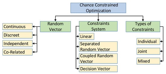
Chance constrained optimization problems can be categorized based on constraints involved as shown in Figure 6. It may have individual, joint, or mixed chance constrained. In individual chance-constrained optimization problems, each element of the stochastic inequality system is transformed into several chance constrained in a unique way where in joint chance-constrained optimization problems, the probability is considered over the stochastic inequality system as a whole. Chance constrained optimization in Equation (4) can be expressed as an individual and joint chance-constrained, as shown in Equations (5) and (6), respectively, [56]. Mixed chance constrained optimization problems may comprize numerous multivariate chance constrained [57]. Individual chance constrained are simple but unreliable compared to joint chance constrained; hence joint chance constrained are used to guarantee the decision at a given probability level [56].

(5)

(6)

Based on the constraints involved in chance constrained optimization problems, it may be linear random vector, separated random vector, coupled random vector, or decision vector. Most important model of chance constrained system is linear random vector. Linear random vector is shown in Equation (4) where the constraint h may adopt different form such as expressed in Equations (7) and (8).

(7)

(8)

where

A (ξ)

and A are stochastic and deterministic matrices, respectively, b is a constant vector of suitable size, g is the function of decision vector x, The model shown in Equations (7) and (8) represents separated and coupled random vector, respectively. In isolated random vector, random vector and decision vector appear separated while combined in the coupled vector model. The random vector may be continuous, discreet, independent or correlated [56].

Figure 6.

Taxonomy of chance constrained optimization.

2. Applications, Objectives and Solution Algorithms of Probabilistic Optimization

2.1. Applications, Objectives and Solution Algorithms of Stochastic Optimization

Applications of stochastic optimization shown in Table 2. Microgrid energy management problems might be seen as having uncertainty in plug-in electric vehicles and distributed renewable energy supplies [58]. The authors in [59] used stochastic dynamic programming to analyse smart home energy management with uncertainty in plug-in electric vehicles. The optimization problem is approached as non-linear programming, and the distribution of electric power among various smart home components is optimized.

Table 2.

Applications of stochastic optimization and its problem type.

References	Applications	LP	NLP	MILP	MISOCP	MIQP

Table 6. Objectives of chance constrained optimization and the solution algorithms.

Objectives of chance constrained optimization and the solution algorithms.

Ref.	Objectives	SAA	AM	SBM	BD and DE	SVM	LR and IM	MDP	MCS	MDP
[59]	HEM		×
[106,130]	Minimize Generation Cost	×	×								[61]	MEM	×
[68]	OPF			×
[62,63]	DRM			×
[23
[67,71,75,81,82,83,84,86,98,110]	Minimize Overall Cost	×	×		×	×		×	×	×
[93]	Minimize Electricity Payment	×					×
[69,87]	Maximize Social Welfare				×				×
[75]	Maximize Profits	×

2.2.1. Smart Grid Energy Management

One of the most common applications of robust optimization is smart grid energy management. Robust optimization can be used to model uncertainty in several parameters. To maximize social welfare, the problem is described as mixed integer linear programming and solved using a consensus algorithm and an optimal control technique [69].

2.2.2. Microgrid Energy Management

The energy management system for single and three-phase balance microgrids is designed using robust convex optimization. The problem is formulated as a mixed integer second-order cone programming [70]. Microgrid energy management takes into account the characteristics and constraints of the system. The system is mathematically modeled using mixed-integer nonlinear programming, which is subsequently linearized using the Lyapunov optimization approach [71]. For microgrid energy management, two-stage adaptive robust optimization is employed while taking into account the uncertainties of renewable energy resources. In both isolated and grid connected modes, the problem is formulated as mixed integer linear programming, and the total operating cost of the system is minimized. The column and constraint creation algorithm efficiently solves the problem [72]. Energy and frequency management of microgrid accomplishes a reliable and robust solution where total cost of the system is minimized by solving mixed integer linear programming using information gap decision theory [73,74].

Microgrid planning uses two-stage robust optimization to reduce operating and maintenance costs, investment costs, emissions, and fuel costs. The composition of a microgrid takes into account both renewable energy sources and dispatchable distributed generation. The key sources of uncertainty are intermittent renewable energy resources and time-varying load, which can be effectively managed by using robust optimization. The column and constraint creation approach aids in the solution of the mixed integer linear programming problem [75]. Scenario-based robust optimization is applied to minimize the microgrid’s social benefit cost by accounting for uncertainty in load and renewable energy resources. Taguchi’s orthogonal array generates scenarios, which are then verified using Monte Carlo simulations [76]. Distributed generation, distributed storage, and distributed economic dispatch are used to manage energy in the microgrid. The Lagrangian relaxation and dual decomposition method is used to reduce the net cost of a microgrid [77].

2.2.3. Unit Commitment

A security constraint unit commitment for the power grid considering the uncertainties in supply and demand is performed. Total operation cost is minimized, and the solution to the problem is achieved by applying the bender’s decomposition and column generation methods [78]. The overall cost of the system gets minimized by applying various algorithms in different domains [79,80]. Unit commitment problem is solved by Benders’ decomposition algorithm [81,82], column and constraints generation algorithm [83,84] and Lagrangian decomposition method [85]. Integrated electricity and heating system is scheduled by column and constraints generation algorithm [86]. Multistage robust optimization is applied for unit commitment, considering the uncertainties of wind power and demand response. The sole objective is to maximize social welfare and to satisfy various constraints. It is being solved by using bender’s decomposition algorithm to achieve unit commitment in an optimal robust way [87].

2.2.4. Demand Side Management

The demand side is scheduled using robust optimization, which takes into account the uncertainty in manually operated appliances. The problem is formulated as quadratic programming [88], where nonlinear programming is used in [89] to minimize the cost of electricity. Commercial building appliances are scheduled in an ideal method to account for the impact of uncertainties. To minimize the cost of power, the optimization problem is framed as a mixed integer linear programming problem.

2.2.5. Smart Home

The robust index method is applied to handle the uncertainties of household load scheduling and minimize the customer discomfort. The problem is mathematically formulated as a mixed integer linear programming which has been solved by using branch and bound algorithm [90]. The proposed model schedules renewable energy resources at the production part and controls the smart home consumption part. An optimal solution achieved, along with the reduction in computational time and electricity cost. Meta-heuristic algorithm is applied to solve the mixed integer linear programming problem [91].

2.2.6. Plugin Electric Vehicles

Bidirectional dispatch coordination of plugin electric vehicles in a power grid restrains the generation cost. The problem is formulated as a mixed integer linear programming and solved by using heuristic approach [92].

2.3. Applications, Objectives and Solution Algorithms of Distributionally Robust Optimization

When considering energy storage, distributed generators, and wind turbines, distributionally robust chance constrained programming is used for energy management of an islanded microgrid. However, using an analytical method, the overall generation cost is minimized [106]. The generation frequency is managed appropriately via quadratic programming, and the generation cost is also curtailed [107].

The unit commitment problem with uncertainty in wind output power is solved via distributionally robust optimization. The MILP optimization problem is solved using an analytical method, and conservatism is reduced by using distribution information. [46,108]. Distance-based distributionally robust optimization is modeled for a unit commitment by using Kullback Leibler divergence. This model handles uncertainties of wind power in the form of an ambiguity set. The problem is arranged as mixed integer non-linear programming and is solved by using bender decomposition and the iterative method. Computational complexities are handled by decomposition method while the iterative algorithm guarantees the global conservatism [109]. The unit commitment problem is solved by Benders’ decomposition algorithm [110].

The authors in [112] applied distributionally robust optimization to solve energy and reserve dispatch problem. It is shown that distributionally robust optimization is a suitable technique for reserve dispatch to fill the gap between stochastic and adjustable robust optimization. Strategic aggregation is offering regulation capacity on behalf of a group of distributed energy resources. Two stage stochastic optimization and distributionally robust chance constrained optimization are utilized for handling the uncertainties in day-ahead and hour-ahead schemes, respectively, [113]. The authors in [114] applied distributionally robust optimization to solve the power flow problem.

2.4. Applications, Objectives and Solution Algorithms of Chance Constrained Optimization

Chance constrained optimization can be applied to a smart power system by considering applications with diverse objectives. Applications and objectives of chance constrained optimization in smart power system are shown in Table 5 and Table 6, respectively.

Table 5. Application of chance constrained optimization and its problem type.

Application of chance constrained optimization and its problem type.

Ref.	Applications	LP	NLP	MIP	MILP	MINLP	MIBLP	MISOCP	SOCP	MIQP
[115,116,117,118,142,143]	MEM	×	×		×	×		×
[129]	HEM				×
,64]
[119,120,121,123,124]	DEM				×		×		×
[127,128]	SDN		×			×
[133]	Constraints Satisfaction		×
[131,132]	Minimize Reserve Cost							×						×		[125,126]	ED		×	DSM

[125]	Minimize Signal Price				×												×
[					142]	Minimize Electricity Cost					×												[24
[141]	PEV
[115,			×
118,134,135]	Minimize Operating Cost						×	×		×							[138]
[116,	ED	×		117				,
119,120,123,127,136,144,148]	Minimize Overall Cost	×	×				×		×			×		×			[130,131,133,134,135,136,137,144]	UC	×	×	×	×		×
[		121]	Minimize Thermal line losses	×
	×														[145]
[128	GEM		×	]	Minimize planning cost
							×						[146]	OPF		×
[139]	Minimize Active Power Losses									×			×				[147]	OPGF		×

[

140

]

Maximize payoff

[145]

Minimize Dispatch cost

[149]

Minimize Social cost

2.4.1. Microgrid Energy Management

Chance constrained optimization for microgrid energy management is used, where uncertainties are considered in various parameters. Electricity cost of microgrid is minimized by using linear programming while satisfying the energy balance constraint [115]. In [116], chance constrained optimization is applied to handle the uncertainties in power exchange between microgrid and macro-grid where overall cost of the system is minimized by using mixed integer linear programming. Chance constrained stochastic cone programming is applied to plan microgrid network and overall system’s cost is minimized. To obtain the solution for the problem, it uses second-order cone programming (SOCP), bi-linear Benders decomposition method, Jensen’s inequalities, and Pareto-optimal cuts [117]. Chance constrained optimization is used for the optimal operation of microgrid having uncertainties where the problem is formulated as a mixed-integer non-linear programming [118].

2.4.2. Distributed Energy Management

In the distribution system, chance constrained optimization helps in the operation and planning of the energy storage system. Overall cost of the system is minimized by using mixed integer linear programming [119,120]. Chance constrained optimization is used to handle the uncertainties that are due to photo-voltaic and batteries. Line losses in the distribution system are reduced by formulating the problem as second order cone programming and solved by analytic method [121,122]. Overall cost of the system is minimized in distributed energy management problem by using mixed integer linear programming [123]. In [124], the authors presented feasibility and profit based planning for the integration of distributed generation. The problem is mathematically formulated as a mixed integer bi-linear programming.

2.4.3. Demand Side Management

Uncertainties due to the consumption pattern and variation in consumers response to the price signal are modeled by chance constrained optimization. The problem is mathematically formulated as non-linear programming to minimize the electricity price and being solved by interior point method [125]. In [126], the authors considered uncertainties due to the interruptable load and consumer response. Penalty to the consumers and variations due to the interrupt-able load are minimized using non linear programming.

2.4.4. Smart Distribution Network

Joint chance constrained optimization handles the high penetration of distributed generator in a distribution network. The support vectors classifier (SVC) identifies zero probability constraints while sampling is done by Monte Carlo Simulations. Overall system cost is reduced by using non-linear programming to formulate the problem [127]. In [128], the authors minimized planning cost where the problem is being formulated as mixed integer non linear programming.

2.4.5. Home Energy Management

Chance constrained optimization for home energy management to optimize the operation of appliances is used. The model to formulate the uncertainties due to electricity prices and fluctuating loads is used. The problem is mathematically modeled as mixed-integer linear programming and being solved by using particle swarm optimization and two-point estimation method [129].

2.4.6. Unit Commitment

The chance constrained two stage stochastic program minimizes the overall generation cost, whereas sample average approximation helps in solving the mixed integer linear programming problem [130]. Spinning reserve cost gets minimized in an uncertain controllable load by using chance constrained optimization. The problems are mathematically formulated as linear programming which are being solved by applying the analytic method and scenario base analysis in [131] and in [132], respectively. Overall system’s cost gets minimized by applying the ranking algorithm, and the iterative method in unit commitment problem using mixed integer linear programming [123]. The authors in [133] applied analytic method to satisfy the constraints in unit commitment problem. Operating cost is minimized by formulating the unit commitment problems as mixed integer programming and mixed integer second order cone programming in [134,135], respectively. Overall cost of the system is minimized in [136] using mixed integer quadratic programming and non-linear programming in [137].

2.4.7. Economic Dispatch

Economic dispatch problem is formulated as a linear programming problem in [138]. Active power losses are minimized in thermostatically controllable load, where Spatio temporal and dual decomposition algorithm solve the problem [139]. The pay-off gets maximized, and the problem is solved by applying linear regression and iterative method [140]. Dispatch coordination for plug-in electric vehicles are modeled as a mixed integer quadratic programming [141].