Pipelines are widely used to transport oil and gas products over long distances. Ensuring pipeline safety is a prerequisite for the transportation of fuels such as oil and natural gas. Researchers are committed to constructing more accurate and effective health management models and improving the integrity management system of pipelines. Researchers ^[1][2][3][1,2,3] summarized the existing models in the field of pipeline integrity management and pointed out that, although the current models consider the accuracy of inline inspection tools, they are still too ideal and challenging to accurately reflect the proper working conditions of the pipeline. Metal-loss corrosion defects are significant threats to pipeline integrity. Some researchers use stochastic processes to describe uncertainties associated with the degradation of wall thickness incurred by corrosion defects. Wang et al. [4] proposed a stochastic corrosion growth model using the geometric Brownian bridge process. Ossai et al. [5] used a non-homogeneous linear growth pure birth Markov model to predict the degradation of internal corrosion defects in oil and gas pipelines. Bazan and Beck [6] employed a Poisson square wave process to describe the corrosion growth rate and compared the proposed non-linear stochastic model with the linear corrosion growth model. Qin et al. [7] proposed a corrosion growth model based on Inverse Gaussian process and Markov Chain Monte Carlo simulation method. Pan et al. [8] also used Inverse Gaussian process to characterize the degradation process of defects. Peng et al. [9] proposed a Bayesian framework of Inverse Gaussian process models. Remaining useful life of pipelines with multiple defects was predicted in refs. ^[10][11][12][10,11,12]. Although these corrosion growth models take multiple corrosion defects into account, they hardly consider the interacting effects among these defects, let alone the interactions between different types of defects.

There are a number of papers investigating pipelines with interacting corrosion defects. Benjamin et al. ^[13][14][13,14] presented a detailed literature review of pipelines with interacting corrosion defects and a database of corroded pipe tests. Amandi et al. [15] proposed a finite element model combined with a curve fitting method to estimate the remaining strength of pipelines with interacting corrosion defects. Sun and Cheng [16] also implemented a 3D finite element model to investigate mechano-electrochemical interaction of multiple longitudinal corrosion defects. Soares et al. [17] presented a model to analyze the integrity of pipelines with interacting corrosion defects under internal pressure and thermal stresses. Chen et al. [18] used a nonlinear finite element model to study the failure pressure of X80 pipelines with interacting corrosion defects. Kuppusamy et al. [19] investigated the effect of interaction of corrosion defects on the buckling strength of pipelines. Assessing and managing crack defects is also a vital part of pipeline integrity management. The remaining useful life prediction for pipelines with a single crack defect was conducted in refs. ^[20][21][22][20,21,22]. As for pipelines with interacting crack defects, Zhang et al. [23] presented a numerical model and fatigue simulations to analyze the fatigue behaviors. The corrosive environment will affect the growth of the crack, which is called Stress Corrosion Cracking (SCC). Hu et al. [24] applied the Monte Carlo method to predict and evaluate SCC. Lu et al. [25] established an SCC crack growth model in a high pH environment and verified it through experiments. Sekhar [26] summarized the effects of various crack interactions. This study shows that it is necessary to include the analysis of the interaction coupling between crack defects. These studies are all about the interaction between different defects of the same type. However, the exploration of interaction impact between different types of defects is still lacking in the existing literature.

In pipelines, common pipeline defects, such as crack and corrosion, exist at the same time. Specifically, there is an interacting effect between the fatigue crack and corrosion defect in the same pipeline segment. Pipeline corrosion will change the strength of the pipeline in the surrounding area. If the corrosion and crack defects are adjacent, a certain interaction coupling will occur and impact the Stress Intensity Factor (SIF) of the crack surface, thereby affecting the propagation of fatigue crack. Therefore, the crack propagation model that considers the interaction between these two types of defects is conducive to formulating more accurate detection and maintenance strategies. Motivated by this need, this paper plans to study the interacting effects of corrosion and crack defects on pipeline crack propagation.

2. The Pipeline Finite Element Analysis Model

2.1. The FEA Model

In this section, the finite element software ANSYS^® is used to model the pipeline with interacting fatigue crack and external corrosion defects. In the modeling process, the pipeline models with and without corrosion defects are established, respectively, to analyze the interaction impact of corrosion defect on crack propagation. The material of the modelled pipeline is API 5L X70. The outside diameter of the pipeline is set as 914.4 mm, and the wall thickness is 15.875 mm. The internal pressure is assumed to be 1 MPa for modeling. The fatigue crack is modeled as a semi-elliptical shape with a length of 15.2 mm and a crack depth in the range of 2 mm–12 mm. The SIF values corresponding to the deepest point and edge point can be obtained through stress analysis. The internal pressure of the pipeline is 1 MPa. At the same time, there are cuboid corrosion defects on the outer surface of the pipeline, and the axial distance from the crack center to the corrosion center moves from 150 mm to 500 mm. The depth of the corrosion defect is from 2 mm to 14 mm, with an increment of 1 mm each time. The geometric modeling of a corroded pipeline is shown in Figure 1, and the finite element model built in this paper is shown in Figure 2.

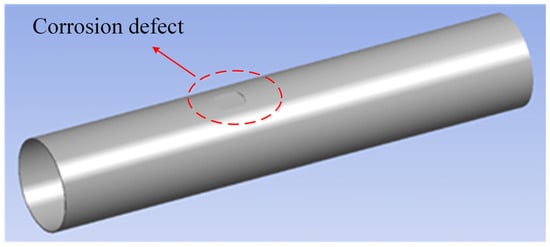
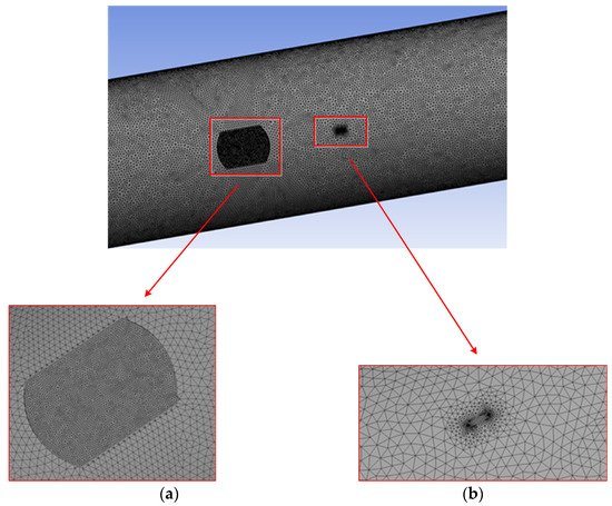
Figure 1. Geometric modeling of corroded pipeline.

Figure 2. The grid division of pipeline. (a) Partial refinement of corrosion defect grid. (b) Partial refinement of grid at crack.

2.2. Validation of FEA

Generally, fracture in engineering structures can be classified into three types: opening mode (I), sliding mode (II) and tearing mode (III), and SIF is used to reflect these modes. Compared with mode II and III, SIF corresponding to mode I is much larger, so the mode I SIF dominates the propagation of fatigue crack. In this paper, mode I SIF was only considered in the pipeline remaining useful life prediction. The method based on API579 for the partial verification of FEA model was employed. According to API579 criterion, the SIF of mode I of the pipeline is calculated as follows:

$$K=\frac{p{R}_i^2\frac{R_o^2-R_i^2\frac{}{}[2G_0+2G_1(\frac{a}{R_o\frac{}{})+3G_2{(\frac{a}{R_o\frac{}{})2^{}+4G_3{(\frac{a}{R_o\frac{}{})3^{}+5G_4{(\frac{a}{R_o\frac{}{}\left)4^{}\right]\sqrt{\frac{\pi a\frac{Q}{}\sqrt{}}{}}}}^{}}}^{}}}^{}}}{}}{}$$

(1)

$$Q=1.0+1.464{\left(\frac{a}{c}\right){1.65{}^{}, for \frac{a}{c}\le 1}^{}}^{}$$

(2)

$$G_0=A_{0,0{}_{}+A_{1,0{}_{}\beta +A_{2,0{}_{}{\beta }^2+A_{3,0{}_{}{\beta }^3+A_{4,0{}_{}{\beta }^4+A_{5,0{}_{}{\beta }^5+A_{6,0{}_{}{\beta }^6}}}}}}}$$

(3)

$$G_1=A_{0,1{}_{}+A_{1,1{}_{}\beta +A_{2,1{}_{}{\beta }^2+A_{3,1{}_{}{\beta }^3+A_{4,1{}_{}{\beta }^4+A_{5,1{}_{}{\beta }^5+A_{6,1{}_{}{\beta }^6}}}}}}}$$

(4)

$$\beta =\frac{2\varphi \frac{\pi }{}}{}$$

(5)

$$G_2=\frac{\sqrt{2Q\sqrt{}\frac{\pi }{}(\frac{16\frac{15\frac{}{}+\frac{1}{3}{M}_1+\frac{16\frac{105\frac{}{}{M}_2+\frac{1}{12\frac{}{}{M}_3)}}{}}{}}{}}{}}}{}$$

(6)

$$G_3=\frac{\sqrt{2Q\sqrt{}\frac{\pi }{}(\frac{32\frac{35\frac{}{}+\frac{1}{4}{M}_1+\frac{32\frac{315\frac{}{}{M}_2+\frac{1}{20\frac{}{}{M}_3)}}{}}{}}{}}{}}}{}$$

(7)

$$G_4=\frac{\sqrt{2Q\sqrt{}\frac{\pi }{}(\frac{256\frac{315\frac{}{}+\frac{1}{5}{M}_1+\frac{256\frac{3465\frac{}{}{M}_2+\frac{1}{30\frac{}{}{M}_3)}}{}}{}}{}}{}}}{}$$

(8)

$$M_1=\frac{2\pi \frac{\sqrt{2Q\sqrt{}\frac{}{}(3G_1-G_0)-\frac{24\frac{5}{}}{}}}{}}{}$$

(9)

$$M_2=3$$

(10)

$$M_3=\frac{6\pi \frac{\sqrt{2Q\sqrt{}\frac{}{}(G_0-G_1)+\frac{8}{5}}}{}}{}$$

(11)

where p is the internal pressure; R_i is the internal radius; R_o is the outer radius; a is the crack depth; Q is a parameter based on crack geometry; G₀, G₁, G₂, G₃, G₄, M₁, M₂, M₃, A_i,j (i ∈ {0,1,2,3,4,5,6}, {j ∈ 0,1}), β are influence coefficients; ϕ is the included angle; c is the half crack length; and K is the mode I SIF.

The finite element simulation results are compared with the SIF results calculated according to API 579 criterion. The results are shown in Figure 3. It can be found from the figure that for the pipeline without corrosion defects, the SIF obtained by finite element simulation is very close to the results of theoretical calculation for a large portion of crack depth range, and the maximum error is less than 5%. The accuracy of finite element simulation is proved. Then, the SIF of pipeline with corrosion defects is studied. As is obtained from Figure 3, for the same crack depth, the SIF of the pipeline with corrosion defects is greater than that without corrosion defects. With the increase in crack depth, SIF also increases gradually. The comparison results demonstrate that there is an interacting impact of corrosion and crack defects on SIF values. Therefore, it is necessary to study the interacting impact between corrosion and crack defects.

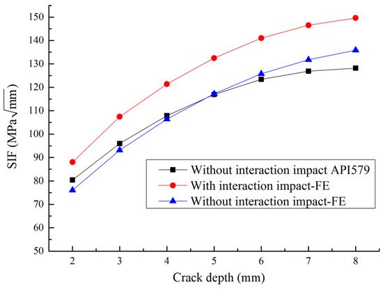
Figure 3. Comparison of pipeline SIF results.