The Compact Muon Solenoid (CMS) is a general-purpose detector at the Large Hadron Collider. The goal of CMS experiment is to investigate a wide range of physics, including the search for the Higgs boson, extra dimensions, and particles that could make up dark matter.
1. Developing a Technique for Measuring the Magnetic Field Inside the CMS Solenoid
The system of the NRM probes installed inside the superconducting solenoid uses the Metrolab Technology SA probes of model 1062, connected through a 2030 multiplexer to a programmable teslameter PT 2025
[1]. The schematic view of the 1062 NMR probe is shown in
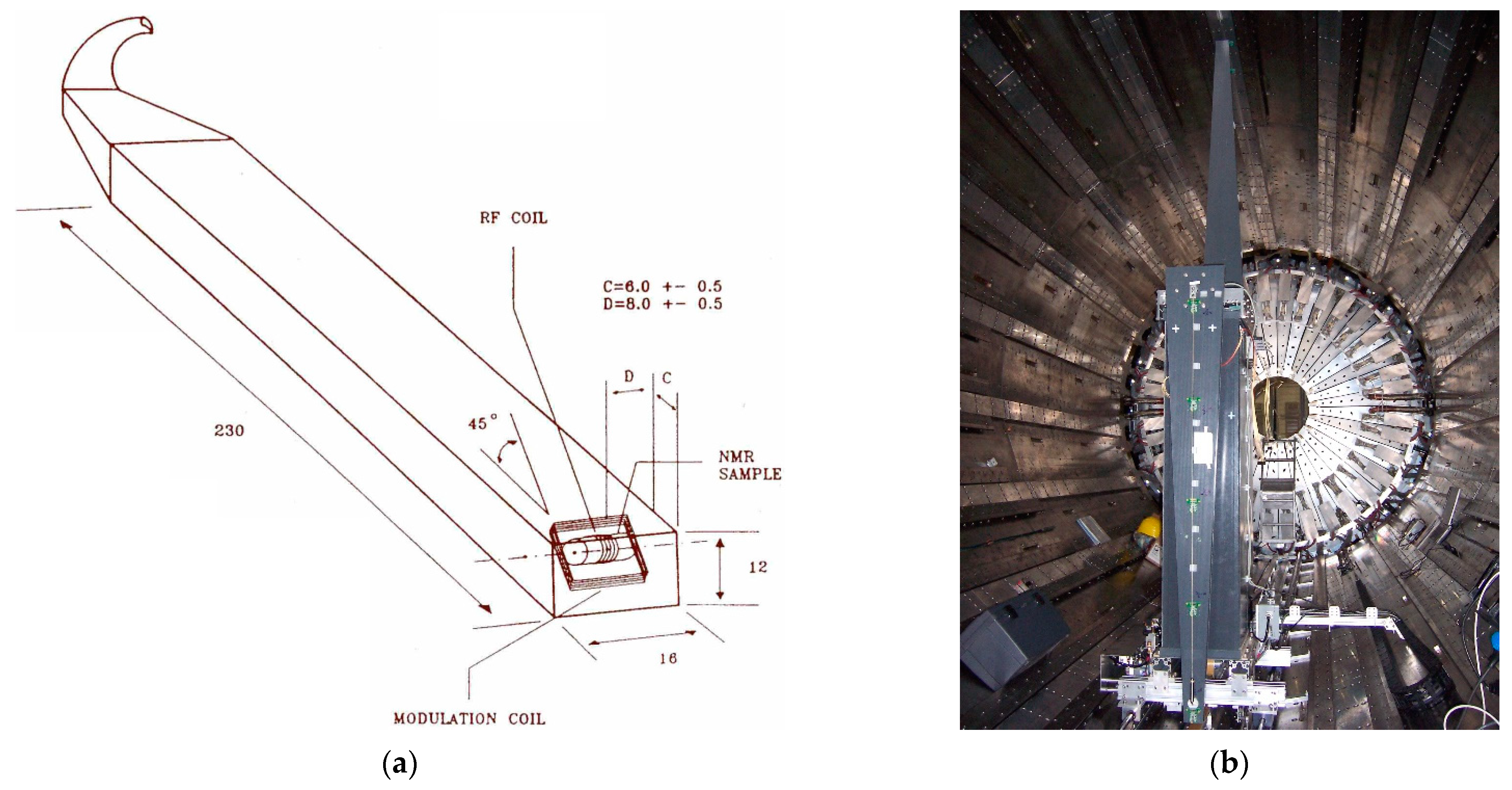
Figure 1a. There are three types of sensors used in the system: one probe (B) has an active volume made of a solid material containing a large amount of hydrogen to measure the magnetic induction in the range from 0.7 to 2.1 T; one probe (F) has a sealed glass tube containing heavy water (D
2O) to measure the magnetic field in the range from 1.5 to 3.4 T; four probes (A, C, D, E) have a similar NMR sample filled with D
2O to measure the magnetic flux density in the range from 3 to 6.8 T. The magnetic field measurement interval is determined by the frequency of the high-frequency generator signal, which is from 30 to 90 MHz for the probe B, from 7.5 to 22.5 MHz for the probe F, and from 15 to 45 MHz for all other probes. This signal is fed to a radio frequency coil located on the active element, and with small perturbation of the strong measuring field by the modulation coil creates conditions for the NMR effect to appear in the active volume, when the oscillation frequency matched the frequency of the nuclear magnetic moment precession around the magnetic field lines and enhances the signal.
Figure 1. (
a) Schematic view of a nuclear magnetic resonance probe. The probe external dimensions in mm (230 × 16 × 12), the position of an active volume (NMR sample) with a radio frequency (RF) coil, as well as the slope of a modulation coil, equal to 45° with respect to the probe axis, are shown. The NMR sample has a diameter of 4 mm and a length of 4.5 mm and is made of either a solid material containing a large amount of hydrogen or a sealed glass tube containing D
2O. The measured magnetic field direction can be transverse or axial; (
b) Automated field-mapping machine
[2] for measuring the CMS magnetic field, installed inside the barrel hadron calorimeter. A carriage made of aluminum alloy moving by steps of 0.05 m along the rails aligned with the
Z-axis, a tower made of durable non-magnetic material, two propeller arms rotating by steps of 7.5° along the azimuth angle in the forward and backward directions, and five 3D B-sensors on the propeller arm viewed from the positive
Z-coordinates are visible.
The modulation frequency of the measured magnetic field is from 30 to 70 Hz and is generated by an additional generator of a triangle signal applied to the modulation coil, the plane of which is located at an angle of 45° with respect to the direction of the measured magnetic flux density, which allows one to measure the transverse or axial magnetic field. Calibration of sensors in a known magnetic field makes it possible to bind the observed oscillation frequency with the value of the corresponding magnetic flux density of the measured field. The combination of the high-frequency and modulation signals provides an accurate magnetic field measurement with a resolution of 0.1 μT (1 Hz in frequency).
The origin of the CMS coordinate system is at the centre of the superconducting solenoid; the X axis lies in the LHC plane and is directed to the centre of the LHC machine; the Y axis is directed upward and is perpendicular to the LHC plane; the Z axis is the right-hand triplet with the X and Y axes and is directed along the vector of magnetic induction generated on the axis of the superconducting coil.
The active volumes of probes A and B are located at a radius of 2.9148 m from the solenoid axis and Z = −0.006 m from the CMS detector median XY-plane at azimuth angles of 44.9° and −135.1°, respectively. The active volumes of probes F and E are located at the same radius and Z = +0.006 m at azimuth angles −44.9° and +135.1°, correspondingly. Probe C measures the magnetic field at a point with coordinates (X, Y, Z) = (0.6425, 0.10517, −2.835) m, and probe D—at a point with coordinates (X, Y, Z) = (0.6425, 0.10517, 2.831) m; both sensors are located at the faces of the tracking system volume.
Teslameter PT 2025 is in the underground service cavern and is connected by three 64-m cables to the 2030 multiplexer located in the underground experimental cavern and connected with 5 NRM sensors by 30-m cables and with one by 35-m cable.
The range of magnetic flux density, B, measured with the NMR probes at the solenoid current values varying from 4 to 19.14 kA, covers the interval from 0.85 to 4.01 T. In this interval, the dependence of B on the solenoid current is linear.
The precise measurement of the magnetic field in the cylinder volume of 1.724 m radius and 7 m long inside the CMS coil has been done in 2006 with a fieldmapper designed and manufactured at FNAL [
8]. The fieldmapper comprised ten 3D B-sensors
[3][4][5] developed at National Institute for Subatomic Physics (Nikhef, Amsterdam, the Netherlands) and calibrated at CERN to a precision of 3 × 10
–4 at 4.5 T field
[6][7][8]. Two NMR probes with the active volumes filled with D
2O were used in addition to measure the field along the coil axis and at the largest radius of the measured volume.
The fieldmapper shown in Figure 1b inside the measured volume moved along the rails installed along the coil axis in the barrel hadron calorimeter, stopping at predefined points where two arms with B-sensors could be rotated through 360°, stopping at predefined angles where the magnetic field was sampled. The azimuth steps were 7.5° in magnitude. Steps along the coil axis were fixed to 0.05 m by a tensioned toothed Kevlar belt.
Each arm of the fieldmapper contained five 3D B-sensors located at radii 0.092, 0.5, 0.908, 1.316, and 1.724 m off the coil axis. The distance between the negative and positive arm B-sensors along the coil axis was 0.95 m.
Made of nonmagnetic materials, the fieldmapper used pneumatic power. The high-purity nitrogen gas flow was controlled with 24-V piezoelectric valves, the remote operation was performed via a programmable logic controller and operator’s LabVIEW
[9] console. The laser ranger was used for absolute
Z-coordinate reference after unscheduled stops.
The alignment of the fieldmapper azimuth axle with respect to the CMS coil axis was performed with a precision better than 1.9 mrad. The read-out of the B-sensors was performed via the CANopen protocol
[10][11].
2. System for Monitoring the Magnetic Flux Density during the CMS Detector Operation
The first stage of the CMS magnetic flux monitoring system consisted of 86 3D B-sensors: 17 high field B-sensors calibrated at 4.5 T magnetic field, and 69 low field B-sensors calibrated at 1.4 T field
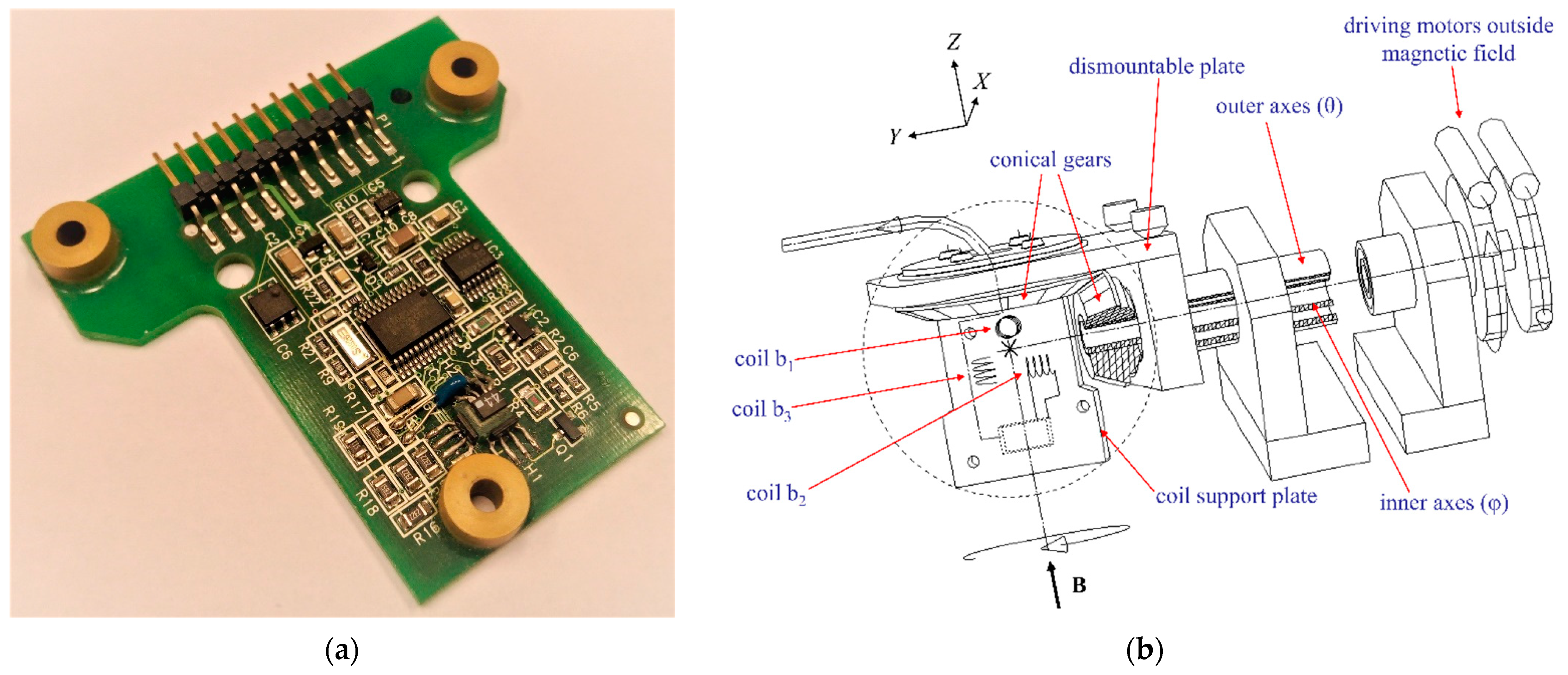
[6][7][8]. The B-sensor printed circuit board (PCB) is shown in
Figure 2a. Three single-axis Siemens GaAs Hall sensors of type KSY44
[12] with dimensions of 3.2 × 2.3 × 0.6 mm
3 each were glued on three orthogonal surfaces of a glass cube with dimensions of 4 × 4 × 2.4 mm
3. The used Hall current was 230 µA, which led to small heat dissipation. Hall voltages were sampled by a 24-bits delta-sigma modulator to perform the signal analogue-to-digital conversion. To measure a temperature nearby the Hall probes a calibrated thermistor is connected to the cube, no thermostat is used. Three precision holes in support legs allow one to mount the PCB on the CMS detector parts. All the PCB analogue electronics resisted the measured field. An 8-byte ID-chip (DS2401 Dallas) on each B-sensor PCB helps to administrate large number of cards in the experiment area.
Figure 2. (
a) Hall probes on the B-sensor PCB. Each PCB contains three single-axis Siemens KSY44 Hall chips
[12] which are glued to a glass cube of 4 × 4 × 2.4 mm
3. The distance between the
b1 (at the cube top) and
b3 (at the H1 side) chip centers is 1.8 mm. The distance between the
b1 and
b2 (at the R18 side) chip centers is 2.6 mm. The B-sensors have an orientation error of about 1 mrad, and the relative orientation error of local
b1,
b2,
b3 measured fields is estimated to be approximately 0.2 mrad
[13]. The analogue voltages from the Hall probes are simultaneously read out by a 24-bit ΔΣ-modulator; (
b) The Hall probe calibrator scheme
[6][7][8]. The local coordinate system
XYZ is rotated with respect to the constant magnetic flux density vector
B in two angular directions: a polar angle
θ is counted between
B and the
Z-axis, and an azimuthal angle
φ is counted between the projection
B·sinθ and the
X-axis. The rotations are performed with the calibrator outer and inner axis providing the rotations of the calibrator head in
θ and
φ directions, accordingly. To cover the full 4
π space in the local reference frame, 6 turns of the outer axis and 5 turns of the inner axis in the opposite directions are needed. Four B-sensor PCB with the same orientation are mounted by two on each side of the coil support plate. Three coils measure the components
b1,
b2, and
b3 of
B in the local coordinate system by the magnetic flux integration. The Hall probe voltages and the coil signals are sampled each 1/15 s and approximated then by the orthogonal spherical harmonics with a set of calibration coefficients at three values of
B and two values of temperature.
A calibration of the 3D B-sensors to a precision of 5 × 10
−4 [14] has been performed by rotation of a package of four PCBs in a constant, homogeneous magnetic field at different absolute field values and temperatures
[6][7][8]. A special calibration device shown in
Figure 2b was designed and manufactured at CERN for this purpose. The calibrator rotated a small head in three constant values of the homogeneous magnetic flux density
B in two orthogonal angular directions
θ and
φ with help of stepping motors located outside the magnetic field and a special transmission consisted of the long inner and outer axis and conical gears. The head was rotated in a thermostat box where a constant temperature was maintained by a Peltier thermoelectric element, and the cooling air flow was controlled by a fan. The middle plate of the head contained three orthogonal coils
b1,
b2, and
b3 to measure the magnetic flux density components by the magnetic flux integration in each coil in the head local reference frame shown in
Figure 2b. On each side of the coil support plate, two B-sensor PCBs were installed.
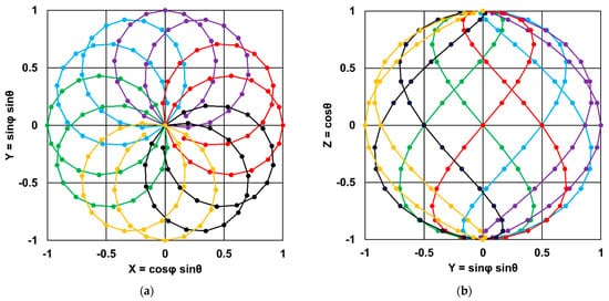
The polar angle θ was counted in the head local coordinate system as an angle between the vector B and the Z-axis. The azimuthal angle φ was counted as an angle between the projection B·sinθ and the X-axis. To complete the full 4π space with rotation of vector B in the local coordinate system, 6 turns of the head in θ-direction and 5 turns of the head in φ direction were needed. A signal/power supply cable winded by the outer (θ) axis but unwinded by the inner (φ) axes. At the end of the calibration, the cable had made only one turn. The trajectories of the magnetic flux density unit vector in the head local reference frame are shown in Figure 3 in the XY- and YZ-planes.
Figure 3. Trajectories of the magnetic flux density unit vector in the calibrator head local coordinate system: (a) in the XY-plane; (b) in the YZ-plane. Different colors correspond to six complete turns of the calibrator head with the outer axes. Markers denote the increments of 9.375° in azimuth φ and 11.25° in polar θ angles used to prepare the plot.
The Hall voltages
VH induced in three single-axis Siemens KSY44 chips during the head rotation have been sampled each 1/15 s together with the coil signals and then were decomposed in orthogonal functions in the way as follows
[7]:
where
cknlm are calibration constants,
Ylm are spherical harmonics
[15] of order
l,
m for spatial part,
Tn are Chebychev polynomials of the first kind
[16] of order
n for temperature dependence,
Tk are Chebychev polynomials of the first kind of order
k for absolute field dependence,
θ and
φ are polar and azimuthal angles,
B is absolute field value, and
t stands for temperature.
A calibration procedure at given magnetic field value and given temperature required three minutes. For a given B-sensor the calibration has been performed for three values of the magnetic flux density (0.37, 0.885, 1.4 T for the low field B-sensors; 2.5, 3, 4.5 T for the high field B-sensors) and for two values of temperature (20 °C and 24 °C). The calibration constants have been stored in the database for each calibrated B-sensor and then were used to convert the measured Hall probe voltages into the magnetic flux density during the magnetic field measurements and monitoring.
3. Developing a Flux Loop Technique of Measurements of the Magnetic Flux Density Inside the CMS Yoke Steel Blocks
3.1. Concept of the Magnetic Flux Density Measurements in Steel with the Flux Loops
A procedure to measure the magnetic flux density inside the CMS yoke steel blocks had been proposed in 2000
[17] and assumed using the fast discharge of the CMS coil to induce voltages in flux loops installed around selected blocks of the CMS flux-return yoke. By sampling the voltage induced in any one loop and integrating the voltage waveform over the time of the discharge, the total initial flux in the loop can be measured. The voltage induced in any one flux loop is proportional to the number of turns in the loop. The average value of the magnetic flux density normal to the plane of the flux loop wound around the block is obtained by dividing the measured value of the magnetic flux by the known area enclosed by the loop and the number of turns in the loop.
The standard ramp up and ramp down time of the CMS magnet is approximately 4–5 h depending on the ramping rate, and the slow discharge time is about 19 h. With a rate of 1.5 A/s, the standard ramp down from an operating current of 18.164 kA to 1 kA takes 11442.7 s. Starting from a current of 1 kA the fast discharge is automatically triggered, and the current decay departs from a simple L/R(t) decay of an inductor (L) into an external resistance (R(t)) changing with time (t), which requires another 3600 s. If the average initial magnetic flux density in the flux loop area of 1 m2 is 1.5 T, then the initial magnetic flux Φ in the loop cross section is 1.5 Wb. Dropping this value to zero for 15,042.7 s induces in one turn of the loop an electromotive force (EMF) voltage V = ∆Φ/∆t of 0.0997 mV. With a loop made of 400 turns the induced voltage reaches 40 mV that requires a precise analogue to digital convertor (ADC) to separate this small signal from a noise. The number of turns was limited by the cross sections of the grooves in steel blocks used for the flux loop arrangements.
The fast discharge time constant is 190 s, which induces voltages with a much larger amplitude. Evidently, measuring the flux loop voltages during coil fast discharge provided the best opportunity to make the intended measurements. During normal operation of the CMS magnet fast discharge of the superconducting solenoid is only triggered by the detection of some abnormal operating condition, which, from a safety point of view, requires discharge of the coil as rapidly as could be achievable. To verify the proper performance of the magnet safety system, several manually triggered fast discharges have been performed in 2006 during commissioning of the CMS magnet [
7] before it was lowered into the CMS underground experimental cavern. These fast discharges provided an opportunity to make the flux loop measurements of the magnetic field in the yoke steel using a simpler ADC.
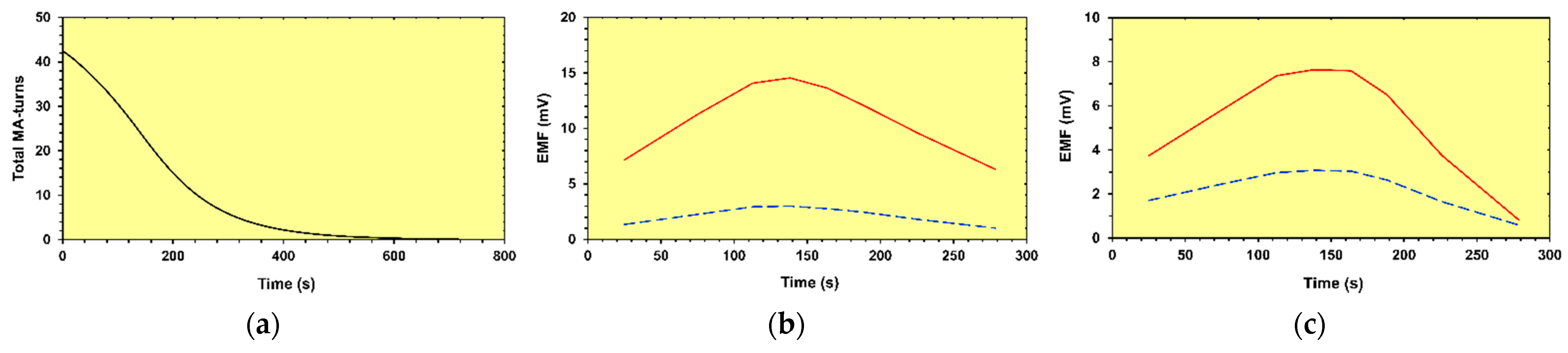
To estimate the amplitudes of signals induced in the flux loops during the fast discharges, the magnetic flux variations in the proposed flux loop displacements have been calculated with the CMS magnet 3D model
[18]. At nine discrete times (0, 50, 100, 125, 151, 176, 200, 251, and 306 s) during the simulated fast discharge shown in
Figure 4a the magnetic flux has been calculated in the entire CMS detector volume. In the blocks of the barrel wheels and the endcap disks, the resulting magnetic flux density values were integrated over the areas enclosed by the flux loops. From the total flux enclosed by each flux loop, the average voltages induced in the loops by the flux changes between time intervals were calculated as shown in
Figure 4b,c. The presence of eddy currents in the steel cores of the flux loops, and their effects on the induced voltages in the loops, have been ignored in the calculations presented in
Figure 4b,c
[18].
Figure 4. Modelled (
a) CMS coil current fast discharge; (
b) minimum (dashed) and maximum (solid) EMF voltages per one-turn flux loop on the blocks of the CMS barrel wheels ; (
c) minimum (dashed) and maximum (solid) voltages per one-turn flux loop on the 18° segments of the CMS endcap disks
[18].
The conclusion of this modelling was that the voltages induced in the flux loops could be integrated with a good precision to obtain the magnetic flux and then the average magnetic induction in the selected cross sections of the CMS flux-return yoke.
According to this study each flux loop was made of 7–10 turns of 45-conductor ribbon cable wound into a shallow groove of 30 mm wide and 12–13 mm deep machined into the peripheral surface of the steel block to be sampled. By connecting the two ends of the loop ribbon cable so that the individual conductors in the ribbon are offset by one conductor, the 315-450-turn flux loops were formed to encircle the selected parts of the yoke. As can be seen in the above-calculated EMF estimates shown in Figure 4b,c, voltages peaking to several volts could be induced in the multiple-turn flux loops.
3.2. Performance of a Special R&D Program to Model the Flux Loop Measurements
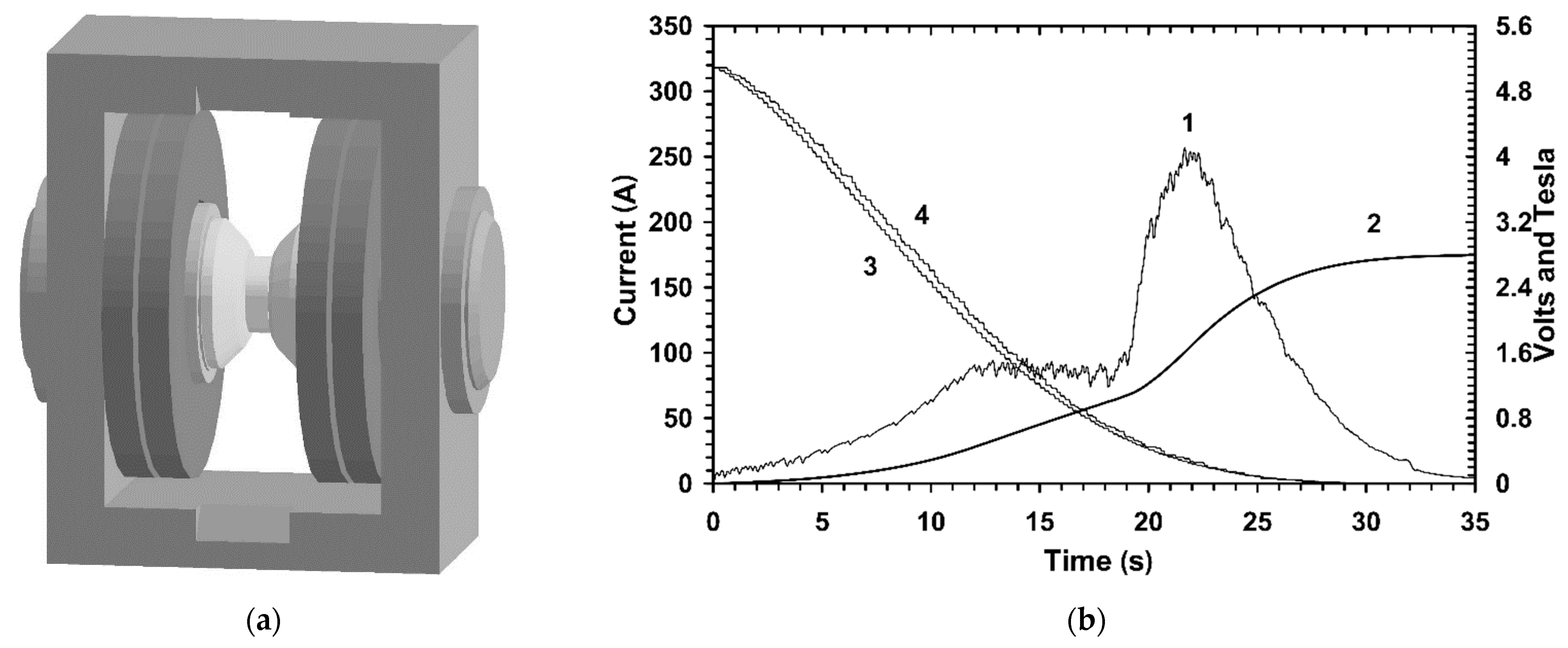
To verify if these voltages can be measured online and integrated offline over the entire CMS fast discharge with an accuracy of a few percent, a special R&D program was performed with several sample disks 127 mm in diameter and 12.7 or 38.1 mm thick made of the CMS yoke steel. Each sample disk was inserted between the poles of a test dipole magnet discharged from a maximum current of 320 A with a current shape similar to the shape of the CMS current generated by the solenoid fast discharge. The induced voltages were measured in a test flux loop mounted on the sample disk. To provide an equivalent variation in the magnetic flux, the number of turns in the test flux loop was larger than the number of turns in the CMS flux loops, and the duration of the test magnet discharge was shorter than the CMS fast discharge time.
The 994-turn test flux loop of 140.6 mm in average diameter was wound on a non-metallic bobbin and connected to the sampling circuitry in differential mode to reject common-mode noise
[18]. The differential inputs of the ADC system were referenced to ground through 100 kΩ resistors.
The test magnet of GMW Associates Model 3474 was energized with Danphysik Model 8530 power supply equipped with General Purpose Interface Bus (GPIB) control interface, and the magnet charging and discharging were performed at several different rates under control by the same software used to sample the voltage on the test flux loop. The diameter of the test flux loop was chosen to fit within the flat portion of the pole tips of the test magnet. A test magnet model shown in
Figure 5a was calculated with the TOSCA program
[19] to interpret the data obtained from the test flux loop. The
B-H curve for the test magnet pole tips and yoke were taken from the measurements of the CMS yoke steel samples.
Figure 5. (
a) 3D model for the test magnet with the steel sample disk inserted between the pole tips
[18]; (
b) Induced voltage (curve 1) and the integrated magnetic flux density (curve 2) when the test magnet current ramped down from 320 A to zero during 32 s. Curve 3 shows the requested current from the control software. Curve 4 corresponds to the measured current read-back
[18].
Numerous sets of measurements were performed with the pole tip gap of the test magnet set to 12.7 mm and 44.45 mm
[18].
In particular, the sample disks of 38.1 mm thickness made of different steel used in the CMS yoke were inserted in a 44.45 mm gap of the test magnet. In these studies, 3.175 mm air gaps between the samples and the pole tips of the test magnet were used to mount the Hall sensors on both sides of the disks at the centers of each side in the air gaps. The Hall sensors measured the axial magnetic flux density on the steel-air interface when the test magnet was fully energized, and the remanent field in the steel at the end of the discharge.
The TOSCA model predicted closely the flux density of 2.65 T in the 12.7 mm free air gap between the pole tips versus that measured by Hall probes (2.63 T) positioned on the surface of the pole tips when the test magnet was energized to full excitation. With the 12.7 mm thick steel sample disk inserted in the gap, the model predicted a field of 3.07 T in the center of the disk.
For the case with the 44.45 mm gap filled with the 38.1 mm steel disk spaced from the pole tips by two air gaps, the model predicted an axial field of 3.0 T in the center of the flat side of the disk when the test magnet is fully energized, whereas the Hall probes measured 2.9397 ± 0.0002 T. Based on this, a correction factor of 0.9799 was applied to other calculated values to be compared with the measured field values.
First, the test flux loop was inserted in the gap of 12.7 mm between the pole tips and the test magnet charged to full current of 320 A at a charge rate of 2.5 A/s. After a pause, the current was decreased at the same rate to zero. The voltage on the test flux-loop was sampled at 50 ms intervals (20 Hz sampling rate), and integrated offline by multiplying the average voltage in each time interval by the length of time interval. The measured flux changes from charging and discharging agreed within 2%.
Then, an aluminum disk 12.7 mm thick was placed in the flux loop and the assembly inserted between the pole tips. The behavior of the voltage induced in the test flux-loop was the same that excluded the substantial eddy currents in the metal sample disks.
The main studies were performed with two 38.1 mm thick sample disks made from the same steel as most of the CMS barrel yoke. Each was inserted into the test flux loop and spaced from the test magnet pole tips by air gaps of 3.175 mm. The charge-up of the test magnet was always at the rate of 2.5 A/s. Fast discharges have been studied with the overall discharge times of 32, 64, 128, 256, and 512 s with the shapes similar to the CMS fast discharge. Figure 5b shows the induced voltage and integrated magnetic flux density for the discharge time of 32 s. Before the charge-up and at the end of the discharge, the Hall probes measured the remanent fields in the air gaps Br ch, and Br dis, respectively. It was observed that these remanent fields increased for longer discharge times. It was 37 mT for 32 s discharges and increased to 59 mT for 512 s discharges. The eddy currents in the test magnet poles caused this effect, and it resulted in a long tail of the induced voltage after the current of the test magnet was set to zero. For all the discharges, this tail was measured during 70 s after t = 0 (after 32–512 s from the beginning of the discharge), where t = 0 represents the time when the current was requested by software control to become zero. In the case of the shortest discharge of 32 s, this tail contributed 1.8% to the integrated voltage. For the 512 s discharge, this contribution was 0.008%. The test magnet charge-up and discharge occurred as a series of small discrete steps in current visible in Figure 5b.
In eleven charge/discharge cycles of varying discharge times the sums Br ch + Bi ch, and Bi dis + Br dis were investigated. In these sums Bi ch is the magnetic flux density obtained from the magnetic flux integrated by the test flux loop during the charge-up of the test magnet, and Br ch is the remanent field measured by the Hall sensors before the charge-up began. The subscript “dis” denotes the same quantities measured during discharges of the test magnet (including 70 s after the current was ramped down to zero) with the Hall sensor value recorded after the discharge. Averaging the results from the eleven different cycles gave the values <Br ch + Bi ch> = 2.8633 ± 0.0018 T for charging and <Bi dis + Br dis> = 2.8583 ± 0.0028 T for discharging. The results agreed within 0.2%.
Taking the TOSCA calculations for the flux loop and scaling by the correction factor of 0.9799, a calculated magnetic flux density of 2.8726 T was obtained. This agreed with <Br ch + Bi ch> within 0.3% and with <Bi dis + Br dis> within 0.5%.
4. Analysis of Eddy Current Distributions in the CMS Magnet Yoke during the Solenoid Discharge
Right after the special R&D program described above was performed, sixteen 315–450-turn flux loops have been installed in azimuthal sector S10 at 270° of the central and two CMS negative side barrel wheels and another six 405–450-turn flux loops had been installed in azimuthal sector S10 of two CMS negative side endcap disks. To estimate the contribution of eddy currents to the voltages induced in the flux loops when the fast discharge of the CMS coil occurs, a special CMS magnet 3D model has been developed and calculated with Vector Fields’ program ELEKTRA (Electromagnetic Analysis)
[20].
Calculations with ELEKTRA, which utilizes a vector potential in the regions where the eddy currents are expected, are very CPU time consuming. To reduce CPU time to a reasonable amount, the CMS yoke was described in a simplified way, the number of finite element nodes in the models was reduced to a reasonable value, the time step varied from 6.25 to 25 s, and the number of output times in the transient analysis of the current decay following the drive function shown in
Figure 4a did not exceed 15
[21]. To perform ELEKTRA analysis of eddy currents in the CMS yoke at 15 output times, 415 CPU hours on a 450 MHz processor machine was required. To meet the batch queue requirements and to vary the time step, the analysis restarted at 50, 100, 150, 200, and 300 s. To analyse the magnetic field distribution in absence of eddy currents at the same output times, 12.3 CPU hours were required.
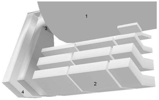
The model shown in
Figure 6 included the entire CMS superconducting coil at cryogenic temperature and a 1/24 segment of the yoke that was then rotated and reflected in the OPERA-3d (an OPerating environment for Electromagnetic Research and Analysis)
[22] postprocessor analysis to obtain the full description of the CMS yoke. This 30° azimuthal segment of the yoke was described as two and one-half three-layered barrel wheels, a small nose disk, and two thick endcap disks. Neither the connection brackets between the barrel layers nor the azimuth gaps in the CMS barrel wheels were modelled. The thin endcap disks and ferromagnetic parts of the CMS forward hadronic calorimeter were also omitted.
Figure 6. ELEKTRA model used for the yoke eddy current calculation
[21]. CMS coil (1), the yoke sectors of the barrel wheels (2), nose disk (3), and two endcap disks (4) are presented in the model.
Different magnetic and electrical properties of materials were used to describe three different regions of the yoke: the tail catcher (TC, an additional inner layer of the central barrel wheel) and the first full-length thin barrel layer (L1) (region 1); second (L2) and third (L3) thick barrel layers (region 2); the nose and endcap discs (region 3).
A vector potential was used in all three regions. The electrical resistivity of construction steel used in calculations in regions 1, 2, and 3 was equal to 0.18, 0.15, and 0.165 µΩ, respectively.
The calculations of eddy currents in the CMS yoke were performed with ELEKTRA at 0, 25, 50, 100, 125, 150, 175, 200, 250, 300, 350, 400, 500, 600, and 700 s from the start of the simulated CMS fast discharge. At the same output times another ELEKTRA analysis was done with the model, which assumes an infinite electrical resistivity and total scalar magnetic potential instead of vector potential in all regions of the yoke.
The maximum eddy current density was investigated in the 22 flux loop steel cores. The calculation indicated that the maximum eddy currents in the yoke barrel cross sections arrived at 140 s after the beginning of the discharge, where the derivative of the current with respect to time reached an extreme. The eddy currents in the yoke endcap disk cross sections reached the maximum approximately 20 s later
[21].
In the TC flux loop core the maximum eddy current density was 2.59 kA/m2. In the L1 flux loop cores the maximum eddy current density varied from 4.16 to 12.9 kA/m2. In similar cross sections of the L2 barrel layer, the maximum eddy current density varied from 5.14 to 12.5 kA/m2. In the cross sections of the L3 barrel layer, the maximum eddy current density varied from 5.42 to 7.38 kA/m2.
In the flux loop cores of the first endcap disk D−1, the maximum eddy current density varied from 27.12 to 51.98 kA/m2 and, in the cross sections of the second endcap disk D−2, the maximum eddy current density varied from 11.21 to 17.52 kA/m2.
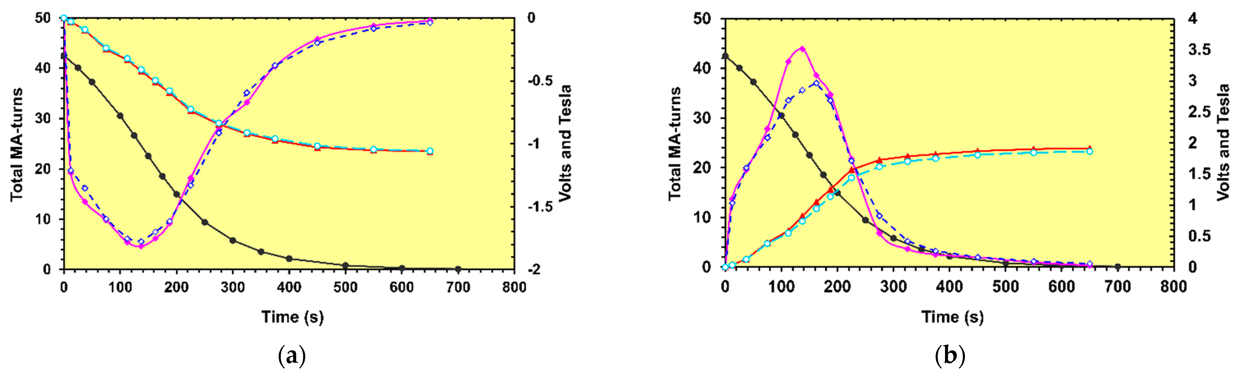
To investigate if these values of the eddy current density change the magnetic flux, and thus, the average magnetic flux density in the yoke cross sections enclosed by the flux loops, the average voltages induced in the flux loops by the magnetic flux changes between time intervals were calculated as shown in Figure 7a,b.
Figure 7. (a) Voltages calculated in the first flux loop on the L2 layer of the external barrel wheel when the eddy currents with realistic electrical resistances (dotted blue line with open diamonds) and infinite resistances (smoothed solid magenta line with filled diamonds) are modelled during the current fast discharge (black solid line with black circles). The dashed light blue line with open circles represents the result of voltage integration when the eddy currents exist. The solid red line with filled triangles displays the result of voltage integration in the model with eddy currents suppressed. The difference between two integrated magnetic flux densities is within 0.3%; (b) Voltages calculated in the middle flux loop on 18° segment of the D−2 endcap disk when eddy currents from realistic electrical resistances (dotted blue line with open diamonds) and eddy currents suppressed by infinite resistances (smoothed solid magenta line with filled diamonds) are modelled during the current fast discharge (black solid line with black circles). The dashed light blue line with open circles represents the result of voltage integration when eddy currents exist. The solid red line with filled triangles displays the result of voltage integration when eddy currents are suppressed. The difference between two integrated magnetic flux densities is within 2.8%.
The voltages obtained in both models were integrated by multiplying the average voltage in each time interval by the length of time interval. The time integrals of the voltages are the total flux changes in the flux loops. The obtained flux values were renormalized to magnetic flux density using the areas of the flux loops and the numbers of turns in the flux loops.
The expected average eddy current contributions were found as follows: 0.22% ± 0.89% in the flux loop cores on the barrel wheels; −0.83% ± 2.42% in the flux loop cores on the endcap disks; and −0.067% ± 1.55% in all the yoke cross sections enclosed by the flux loops. A minus sign indicates that the value of the average magnetic flux density integrated in the model with eddy currents is less than the same value in the model without eddy currents.
These contributions lay well within the expected uncertainties of 2–3% anticipated in the flux coil measurements of the average magnetic flux density in steel elements of the CMS yoke, as was determined in the special R&D program
[23].