1. Introduction

Thermodynamics is an empirical physical theory which describes relevant aspects of the behavior of macroscopic systems. In some form or another, all large physical systems are shown to satisfy this theory. It is based on two most relevant concepts, namely energy. The German physicist and mathematician Rudolf Julius Emanuel Clausius (1822–1888) introduced the concept of entropy in 1865 ^[1][2][1,2], along rather abstract lines in fact. He coined the word from the Greek τροπη (trope¯ )(trope¯), meaning transformation, turning, change. Clausius seemingly appreciated the phonetic and etymological consonance with the word ’energy’ itself, from the Greek ευεργεια (energeia), meaning activity, operation, work. It is generally believed that Clausius denoted the entropy with the letter S in honor of the French scientist Sadi Carnot. For a reversible infinitesimal process, the exact differential quantity dS is related to the differential heat transfer δQreversible through dS = δQreversible /T , T being the absolute temperature. The quantity T^{-1 plays the role of an integrating factor, which transforms the differential transfer of heat (dependent on the specific path of the physical transformation) into the exact differential quantity of entropy (path-independent). This relation was thereafter generalized by Clausius into its celebrated inequality} dS ≥ δQ/T, the equality corresponding to a reversible process. The inequality corresponds to irreversible processes and is directly implied by the so-called Second Principle of Thermodynamics, deeply related to our human perception of the arrow of time.

One decade later, the Austrian physicist and philosopher Ludwig Eduard Boltzmann (1844–1906) made a crucial discovery, namely the connection of the thermodynamic entropy S with the microscopic world  ^[3][4][3,4]. The celebrated formula S = k ln W, W being the total number of equally probable microscopic possibilities compatible with our information about the system, is carved in his tombstone in the Central Cemetery of Vienna. Although undoubtedly Boltzmann knew this relation, it appears that he never wrote it in one of his papers. The American physicist, chemist and mathematician Josiah Willard Gibbs (1839–1903) further discussed and extended the physical meaning of this connection ^[5][6][7][5–7]. Their efforts culminated in the formulation of a powerful theory, currently known as statistical mechanics. This very name was, at the time, a deeply controversial matter. Indeed, it juxtaposes the word mechanics—cornerstone of a fully deterministic understanding of Newtonian mechanics—and the word statistics—cornerstone of a probabilistic description, precisely based on non-deterministic concepts. On top of that, there was the contradiction with the Aristotelian view that fluids, e.g., the air, belong to the mineral kingdom of nature, where there is no place for spontaneous motion. In severe variance, Boltzmann’s interpretation of the very concept of temperature was directly related to spontaneous space-time fluctuations of the molecules (‘atoms’) which constitute the fluid itself.

Many important contributions followed, including those by Max Planck, Paul and Tatyana Ehrenfest, and Albert Einstein himself. Moreover, we mention here an important next step concerning entropy, namely its extension to quantum mechanical systems. It was introduced in 1927 [8] by the Hungarian-American mathematician, physicist and computer scientist János Lajos Neumann (John von Neumann; 1903–1957).

The next nontrivial advance was done in 1948 by the American electrical engineer and mathematician Claude Elwood Shannon (1916–2001), who based on the concept of entropy his “Mathematical Theory of Communication” ^[9][10][11] [9–11]. This was the seed of what nowadays is ubiquitously referred to as the information theory, within which the American physicist Edwin Thompson Jaynes (1922–1998) introduced the maximal entropy principle, thus establishing the connection with statistical mechanics ^[12][13] [12,13]. Along these lines, several generalizations were introduced, the first of them, hereafter noted SqR, by the Hungarian mathematician Alfréd Rényi (1921–1970) in 1961 ^{[14][15][16][17]}[14–17]. Various others followed in the next few decades within the realm of information theory, cybernetics and other computer-based frames, such as the functionals by Havrda, Charvat ^[18] [18], Lindhard, Nielsen ^[19] [19], Sharma, Taneja, Mittal ^[20][21][22][20–22]. During this long maturation period, many important issues have been punctuated. Let us mention, for instance, Jaynes’ “anthropomorphic” conceptualization of entropy ^[23] [23] (first pointed by E.P. Wigner), and also Landauer’s “Information is physical” ^[24] [24]. In all cases, the entropy emerges as a measure (a logarithmic measure for the Boltzmann–Gibbs instance) of the number of states of the system that are accessible, or, equivalently, as a measure of our ignorance or uncertainty about the system.

In 1988, the Greek-Argentine-Brazilian physicist Constantino Tsallis proposed the generalization of statistical mechanics itself on the basis of a nonadditive entropy, noted Sq, where the index q is a real number; Sq recovers the Boltzmann–Gibbs (BG) expression for the value q = 1 ^[25] [25]. This theory is currently referred to as nonextensive statistical mechanics [26]. There was subsequently an explosion of entropic functionals: there are nowadays over fifty such entropies in the available literature. However, very few among them have found neat applications in physics and elsewhere.

2. Basics

2.1. Definitions and Properties of Entropy

The Boltzmann–Gibbs–von Neumann–Shannon entropic functional (or entropy for simplicity) for discrete variables is defined as follows:

where k is a conventional positive constant (currently taken to be the Boltzmann constant in physics, and k = 1 in information theory), and {pi} are the probabilities corresponding to W possible states.

For classical systems, the discrete index i is replaced by a real continuous variable x, and we have the form that was used by Boltzmann and Gibbs themselves, namely

(Some mathematical care might be necessary in this limiting case; for instance, if the distribution is extremely thin, this classical expression of SBG might lead to unphysical negative values; although not particularly transparent, such difficulties simply disappear if we take into account that the Planck constant is different from zero.)

For quantum systems, we have

where ρ is the density matrix, acting on an appropriate Hilbert space; under this form, SBG is also referred to as von Neumann entropy [8]. Definition (1) can be expressed as a particular instance of (2) through Dirac’s delta distributions (with p(x) = ∑^W_{i=1 δ}(xi - pi)), and also as a particular instance of (3) when ρ is diagonal.

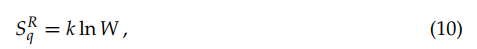
In all cases, we may say that entropy is a logarithmic measure of the lack of information on the system. When we know everything about the state of the system (more precisely, on which one of the possible W states the system is), SBG vanishes. When we know nothing (more precisely, when pi = 1/W for all values of i) SBG attains its maximal value

This equality constitutes a crucial connection between the macroscopic world (represented by the thermodynamical entropy SBG) and the microscopic world (represented by the total number W of microscopic possibilities).

Let us now address the generalizations of SBG that exist in the literature. Given their enormous amount, we shall restrict ourselves to the two most popular ones after the BG entropy itself, namely the additive Renyi entropy SR_q [14–17] and the nonadditive entropy Sq [25]. They are respectively defined as follows, q being a real number:

and

where the q-logarithmic function is defined through

The quantity σ(p) ≡ ln(1/p) is referred to as surprise [27] or unexpectedness [28]. It vanishes when the probability p equals unity, and diverges when the probability p→0. We can consistently define q-surprise or q-unexpectedness as σq(p) ≡ lnq(1/p), hence σq(1) = 0 and σq(0) diverges. With this definition, Sq can be rewritten in the following way:

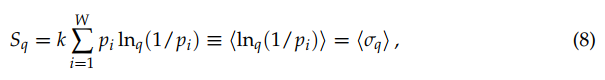where ‹.› denotes the mean value.

It can be verified that

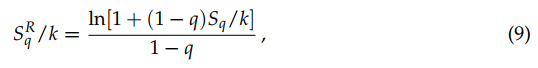
which implies that S_q^R monotonically increases with Sq (like, say, (SBG)^{3 monotonically increases with} SBG). Moreover, it can be shown that Sq({pi}) is concave for q > 0, and convex for q < 0, whereas S_q^R is concave for 0 < q ≤ 1, convex for q < 0, and neither concave nor convex for q > 1. They both attain, for equal probabilities, their extremal value (maximal for q > 0, and minimal for q < 0), namely

and

2.2. Additivity versus Extensivity

We address now two important notions, namely entropic additivity and extensivity. Following O. Penrose [29], an entropic functional S({pi}) is said additive if, for two probabilistically independent systems A and B (i.e., p_ij ^A+B = p_i^Ap^B_j ), we verify S(A + B) = S(A) + S(B), in other words, if we verify that

Otherwise, S({pi}) is said nonadditive. It immediately follows that SBG and S_q^R (for all values of q) are additive. In contrast, Sq satisfies

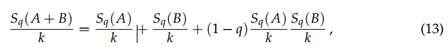
hence

Therefore, unless (1 - q)/k→0, Sq is nonadditive.

Let us briefly mention at this point a simple generalization of Sq which appears to be convenient for some specific purposes, such as black holes, cosmology, and possibly other physical systems. We define [30]

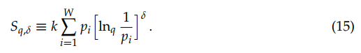
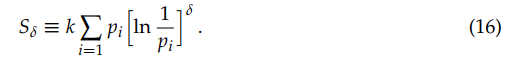
We can verify that S1,1 = SBG, Sq,1 = Sq, and S1,δ = S_δ where [26,31]

Various properties of the nonadditive entropy Sq,δ are discussed in [32].

Let us now address the other important entropic concept, namely extensivity. An entropy S(N) is said extensive if a specific entropic functional is applied to a many-body system with N = Ld particles, where L is its dimensionless linear size and d its spatial dimension, and satisfies the thermodynamical expectation

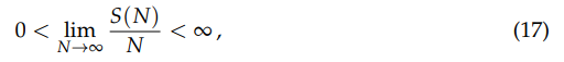
hence S(N) ∝ N for N≥1. Therefore, entropic additivity only depends on the entropic functional, whereas entropic extensivity depends on both the chosen entropic functional and the system itself (its constituents and the correlations among them).

Let us illustrate this distinction through four, among infinitely many, equal-probability typical examples of W(N) (N→∞), where W is the total number of possibilities whose probability does not vanish.

• Exponential class W(N) ∼ A_μN (A > 0; μ> 1):

This is the typical case within the BG theory. We have SBG(N) = k ln W(N) ∼N ln  μ+ ln A ∝ N, therefore SBG is extensive, as thermodynamically required.

• Power-law class W(N) ∼ BN^ρ (B > 0; ρ > 0):

We should not use SBG since it implies SBG(N) = k ln W(N) ∼ ρ ln N + ln B ∝ ln N, thus violating thermodynamics. We verify instead that Sq=1-1/_ρ(N) = k lnq=1-1/ρ W(N) ∝ N, as thermodynamically required.

• Stretched exponential class W(N) ∼ C_νNγ (C > 0; ν > 1; 0 < γ < 1): In this instance, no value of q exists which would imply an extensive entropy Sq. We can instead used S_δ with δ = 1/γ. Indeed, Sd=1/γ(N) = k[ln W(N)]^δ ∝ N, as thermodynamically required.

• Logarithmic class W(N) ∼ D ln N (D > 0):

In this case, no values of (q,δ) exist which imply an extensive entropy Sq,d. Instead, we can use the Curado entropy [33] S_λ^{C(N) = k[eλW(N) - eλ] with λ = 1/D. Indeed, we can verify that SC_λ=1/D(N) ∝ N, as thermodynamically required.}

These four paradigmatic cases are indicated in Figure 1.

It is pertinent to remind, at this point, Einstein’s 1949 words [34]: “A theory is the more impressive the greater the simplicity of its premises is, the more different kinds of things it relates, and the more extended is its area of applicability. Therefore the deep impression that classical thermodynamics made upon me. It is the only physical theory of universal content concerning which I am convinced that, within the framework of applicability of its basic concepts, it will never be overthrown”.

To better understand the strength of these words, a metaphor can be used. Within Newtonian mechanics, we have the well-known Galilean composition of velocities ν13 =[ν12 +ν23]. In special relativity, this law was generalized into v13 = [ν12 +ν23]/[1+ν12ν23/c²]. Why did Einstein abandon the simple linear composition of Galileo? Because he had a higher goal, namely to unify mechanics and Maxwell electromagnetism, and, for this, he had to impose the invariance with regard to the Lorentz transformation. We may thus see the violation of the linear Galilean composition as a small price to pay for a major endeavor. Analogously, what is expressed in Figure 1, is that generalizing the linear composition law of SBG with regard to independent systems into the nonlinear composition (13) may be seen as a small price to pay for a major endeavor, namely to always satisfy the Legendre structure of thermodynamics. However, it is mandatory to register here that such a viewpoint is nevertheless not free from controversy, in spite of its simplicity. For example, the well-known expression of Bekenstein and Hawking for the entropy for a black hole is proportional to its surface instead of to its volume, therefore violating the above requirement.

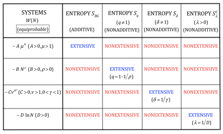
Figure 1. Typical behaviors of W(N) (number of nonzero-probability states of a system with N random variables) in the N→∞ limit and entropic functionals which, under the assumption of equal probabilities for all states with nonzero probability, yield extensive entropies for specific values of the corresponding (nonadditive) entropic indices. In what concerns the exponential class W(N) ∼ A_μ^N, SBG is not the unique entropy that yields entropic extensivity; the (additive) Renyi entropic functional S^Rq also is extensive for all values of q. Analogously, in what concerns the stretched-exponential class W(N) ∼ C_νNγ, the (nonadditive) entropic functional Sd is not unique. All the entropic families illustrated in this table contain SBG as a particular case, except S^C_λ, which is appropriate for the logarithmic class W(N) ∼ D ln N. In the limit N→∞, the inequalities μ^N≥ν^Nγ ≥N^ρ  ln N≥1 are satisfied, hence

This exhibits that, in all these nonadditive cases, the occupancy of the full phase space corresponds essentially to zero Lebesgue measure, similarly to a whole class of (multi) fractals. If the equal probabilities hypothesis is not satisfied, specific analysis becomes necessary and the results might be different.

2.3. Range of Interactions

Let us consider a d-dimensional classical many-body system with say attractive twobody isotropic interactions decaying with a dimensionless distance r ≥ 1 as -A/r^α (A > 0, α ≥ 0), and with a infinitely repulsive potential for 0 ≤ r ≤ 1. At zero temperature T, the total kinetic energy vanishes, and the potential energy per particle is proportional to ∫₁^∞drr^dr^-α. This quantity converges if α/d > 1 and diverges otherwise. These two regimes are from now on respectively referred to as short-range and long-range interactions: see Figure 2.

In addition, they can be shown to respectively correspond, within the BG theory,

to finite and divergent partition functions. This is precisely the point that was addressed by Gibbs himself [5–7]: “In treating of the canonical distribution, we shall always suppose the multiple integral in Equation (92) [the partition function, as we call it nowadays] to have a finite value, as otherwise the coefficient of probability vanishes, and the law of distribution becomes illusory. This will exclude certain cases, but not such apparently, as will affect the value of our results with respect to their bearing on thermodynamics. It will exclude, for instance, cases in which the system or parts of it can be distributed in unlimited space [.]. It also excludes many cases in which the energy can decrease without limit, as when the system contains material points which attract one another inversely as the squares of their distances [.]. For the purposes of a general discussion, it is sufficient to call attention to the assumption implicitly involved in the formula (92)”.

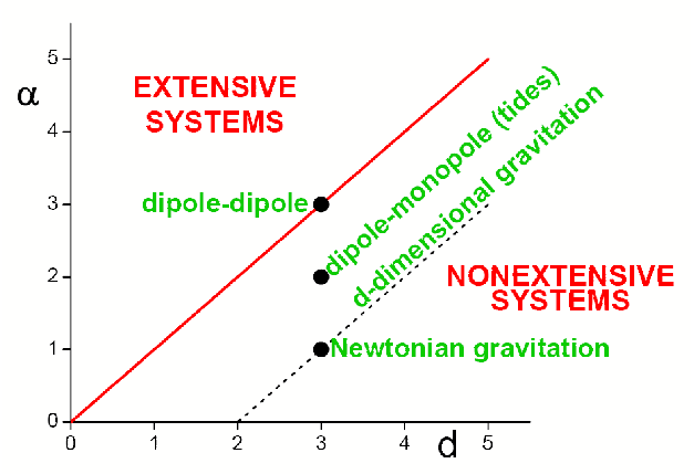
Figure 2. The classical systems for which α/d>1 correspond to an extensive total energy and typically involve absolutely convergent series, whereas the so-called nonextensive systems (0≤α/d<1 for the classical ones) α/d>1correspond to a superextensive total energy and typically involve divergent series. The marginal systems (α/d=1 here) typically involve conditionally convergent series, which therefore depend on the boundary conditions, i.e., typically on the external shape of the system. Capacitors constitute a notorious example of the α/d=1 case. The model usually referred to in the literature as the Hamiltonian-Mean-Field (HMF) one [35] lies on the α=0 axis (for all values of d>0). The models usually referred to as the d-dimensional α-XY [36], α-Heisenberg [37–39] and α-Fermi-Pasta-Ulam (or α-Fermi-Pasta-Ulam-Tsingou problem [40,41]) [42–44] models lie parallel to the vertical axis at abscissa d (for all values of α≥0). The standard Lennard-Jones gas is located at (d,α)=(3,6). From [33].