Your browser does not fully support modern features. Please upgrade for a smoother experience.
Please note this is a comparison between Version 1 by Nasser Shahsavari-pour and Version 2 by Jason Zhu.
Air pollution is one of the major issues in urban management. Researchers proposes a simulated model of the pollution level of the capital city of Tehran along with its source and outcomes based on system dynamics.
- air pollution
- sustainable city
- system dynamics
1. Introduction
Air is vital for the maintenance of human life and also necessary for other creatures on planet Earth. Without air, no one could ever keep on living for more than a few minutes. Air is made up of gases such as nitrogen, oxygen, carbon dioxide, and other gases [1][2][1,2]. A slight change in its composition may result in unpleasant atmospheric conditions for humans and the environment around them. This is called air pollution. Air pollution is a serious environmental issue, particularly in developing countries.
The path of air pollution in the city involves emission and expansion of air pollutants resulting from various factors. Throughout the path, air pollutants are dispersed via various dispersion pathways (air, water, soil, living organisms) thinning and undergoing chemical reactions [3]. In other words, the phenomenon of air pollution is a series including various events such as generation and dispersion of the pollutants from their source, their conversion, transmission, and emission into the atmosphere, and their impact on humans, materials, and the ecosystem [4]. Additionally, air pollution is a major health issue in developing countries. Despite better air quality in the last 50 years, air pollution still reduces the life span of humans and causes a large number of people to go to hospitals. It also causes much harm to the natural environment such that frequent studies indicate that people notice air pollution constantly, especially in urban and industrial regions. Furthermore, epidemiological studies in the last two decades have shown that air pollution is one of the leading causes of death [5]. On the other hand, industrialization and population growth play the main role in air pollution. Air pollution is attributed to an increase in the concentration of greenhouse gases (air pollutants).
System dynamics is a means which helps us to focus on complex problems such as delays, feedback, and nonlinearity. System dynamics with its own development is a field of study which can include science, education, engineering, or medicine. Dynamic modeling consists of four stages, briefly as: (A) conceptualization: defines the purpose of the model and the boundaries, identifies the key variables of the model, describes the behavior or draws reference modes of the key variables, and graphs the basic mechanisms, feedback loops, and system; (B) formulation: involves converting feedback diagrams into level and rate equations, and estimating and selecting the values of the parameters; (C) testing: includes simulation of the model and testing the dynamic hypothesis, testing the model’s assumptions, and testing model behavior and sensitivity to perturbations; and (D) implementation: includes testing the model’s response to different policies, and translating the study insights into one accessible form [6][18].
The use of system dynamics to study environmental systems has gained interest in recent years. In 2010, a study was conducted on Suzhou water resources in China which addressed modeling of water carrying capacity of water resources from 2001 to 2030, in which optimization plans for three water resources were examined [7][19]. In 2012, another survey addressed the interactions between water resources and environmental flow, as well as economic and social status, which was aimed at the evaluation of socio-economic effects of various levels of environmental flows allocation in the Vihe River Delta in China [8][20]. Another study was carried out in China in the same year in which a hybrid approach made of genetic algorithm and system dynamics was considered to measure the pollution burden of coal production on the environment. The genetic algorithm was applied to optimize the system dynamics parameters [9][21]. Moreover, research was conducted in Spain in 2013 which used system dynamics to design a model to study the fate of persistent organic pollutants in soil. The simulation results indicated that the amount of linden in soil had decreased over a 10-year simulating process [10][22]. Bastan et al. showed how a system dynamics simulation approach can provide deep insights into the field of sustainable development and present efficient policies for agricultural sustainability [11][23].
The major part of learning and understanding of how systems and processes work is to observe them while they are in progress. To truly understand the causal loop relations of a system, one should purposefully change the system’s inputs and check the results in the output. In other words, experiments should be done in a way in which each experiment is regarded as a test. Design of experiments is a means in the scientific and engineering world in order to improve the product realization process which is used for evaluation and comparison of basic design configuration, evaluation of material alternatives, and determination of key product design parameters, which affect product performance. Its stages include (1). recognition of and statement of the problem; (2). selection of the response variable; (3). choice of factors, levels, and ranges; (4). choice of experimental design; (5). performing the experiment; (6). statistical analysis of the data; and (7). conclusions and recommendations [12][24].
The capital city of Tehran, with a population of over 8,000,000, has been suffering from severe air pollution due to fast environmental developments in the last couple of years [13][25]. Hence, it seems quite necessary to create a dynamic model aiming at examining the impact of various factors in the city’s air pollution. This article is aimed at building such a model. Then, with the statistical method of design of experiments (DoE), the sensitive and controllable variables are set for the city’s pollution and eventually, plans are offered to reduce the air pollution and several scenarios are proposed to reduce Tehran’s air pollution for a better life.
2. Proposed Method
This paper uses system dynamics to synthesize a simulated model of the polluted capital city of Tehran. It’s different implementing stages are as follows:
-
Stage 1. Defining the dynamic hypotheses.
-
Stage 2. Drawing a causal loop diagram for the system of greenhouse gases emissions in Tehran.
-
Stage 3. Drawing a stock-flow diagram of the system of greenhouse gases emissions in Tehran.
-
Stage 4. Compiling and formulating a model of the system of greenhouse gas emissions in Tehran in mathematical form, which shows interactions inside the system.
-
Stage 5. Identifying critical variables through the statistical method of design of experiments.
-
Stage 6. Demonstrating the output of the model based on optimal values.
-
Stage 7. Defining scenarios for reducing greenhouse gases based on optimized values.
Data for this model were collected from government sites and the model was constructed using causal loops designed based on dynamic hypotheses defined by field experts.
2.1. Causal Loop Diagram
The causal loop diagram is a simple map which shows the relations between the variables by means of arrows relating the cause to the effect. Additionally, the causal loop diagram is a system theory loop which is composed of two balance and reinforcement circles. In the causal loop diagram, the arrows with a mark of “+” are used for the direct relationship between causal loop and those with a minus mark “−” are applied for an inverse relation between causal loop [6][18].
This article represents Tehran’s air pollution in three loops which will be discussed below. It is necessary to first explain the micro-loops to demonstrate the causal loop diagram. That is why micro-loops are brought forward initially and then the causal loop diagram of the entire system will be illustrated. The diagram in Figure 1 represents the causal diagram of the cars which increases once the number of cars grows. Once the cars are totally gone out of the order (junk or scrapped cars) annually, the number of cars reduces.
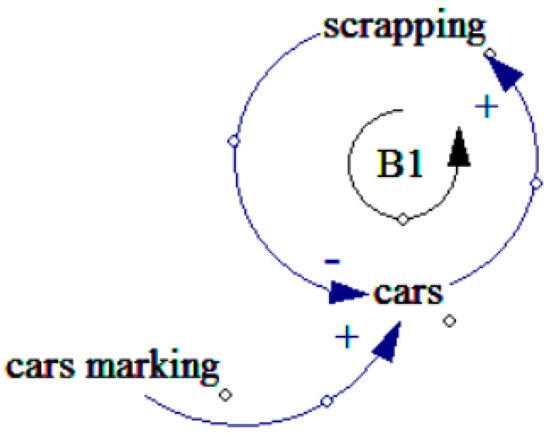
Figure 1. Cars loop.
Figure 2 demonstrates the circle of a number of non-industrial units in which the units grow once the constructions get a license to expand. After their lifetime, a period of 20 years, they suffer total damage and get out of the circle.
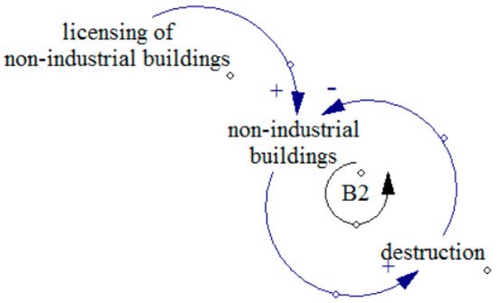
Figure 2. Non-industrial units loop.
Figure 3 illustrates the circle of population variable; when the birth rate increases the population increases. It reduces by natural death and mortality due to pollution.
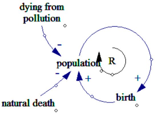
Figure 3. Population loops.
Figure 4 shows a causal loop diagram for the whole system. As demonstrated, pollution grows when the pollutants are dispersed. In fact, some of them are destroyed as a result of natural factors and the remaining causes’ deaths.
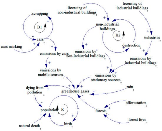
Figure 4. Causal loop diagram for the climate pollution in Tehran.
2.2. Stock-Flow Diagram
Although the causal loop diagrams involve many benefits, in some situations, they also have weaknesses such as the inability to show the stock-flows of the system. This is why stock-flows along with feedback are two central concepts in system dynamics theory.
The stock-flow diagram includes three basic elements: stock, flow, and converters [6][18]. Stocks suggest accumulations inside the system and its stagnation. Flows indicate stocks deviations for input and output. Finally, converters are auxiliary variables to better visualize variables and adjust flows behaviors [6][18].
The boxes in the diagram represent stock variables and faucets show input and output flows. Auxiliary variables are marked with no sign in the graph and are simply represented with their own names. Then, in Figure 5, the diagram is presented.
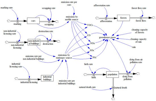
Figure 5. Stock-flow diagram of Tehran’s air pollution.
2.3. Compiling and Formulating the Model and Developing a Mathematical Method
The model contains five stock variables defined using the following Equations:
C = INTEG (M-S, 6,534,000)
M = MR
MR = 398,399
S = C*SR
SR = 1/20
EMS = C*ERC
ERC = 0.0919765
NL = BR
NL = BR
NLR = 31,091.5
D = DR*NB (
DR = 1/25
IB = INTEG (IL, 4075)
IL = ILR
ILR = 48
ESS = (EIB*IB) + (ENB*NB)
EIB = 19.341
ENB = 0.046036
VOCs = ((71,944/613,834)*EMS) + ((11,696/107,927)*ESS)
Co = ((494,201/613,834)*EMS) + ((12,489/107,927)*ESS)
NOx = ((39,430/613,834)*EMS) + ((46,094/107,927)*ESS)
Sox = ((2326/613,834)*EMS) + ((35,085/107,927)*ESS)
PM = ((5933/613,834)*EMS) + ((2563/107,927)*ESS)
GG = (CO + NOx + PM + Sox + VOCs) − ((CCF*F)+(CCR*R))
F = INTEG (A − FF, 6452)
A = AR
AR = 93.583 (
FF = FFR
FFR = 10.25
CCF = 68
R = 23
CCR = 1989
POP = INTEG (B-ND-DP, 8.29314 × 10⁶)
B = BR*POP
BR = 0.014616
ND = DR
DR = 39,317
DP = PO*DPR
DPR = 1/51.318
Note that the first stock variable denotes the number of cars and Equation (1) represents this number in 2011. Equation (2) represents the input flow to the car variable, which is equal to the rate of cars per year. The corresponding number in 2011 is represented by Equation (3). Equation (4) represents the car stock which equals the number of cars multiplied by the rate of scrapped (or junk) cars. The corresponding value in 2011 is represented by Equation (5). Equation (6) depicts the amount of pollutants generated by cars which is the number of cars multiplied by the pollution rate of each car, the value in 2011 of which is given by Equation (7). Equally, Equation (8) relates to the stock variable of non-industrial buildings along with the corresponding value in 2011. Equation (9) shows the input variable of non-industrial buildings which equals the number of issued licenses and permits per year. The corresponding value in 2011 is given in Equation (10). Equation (11) shows the output variable of non-industrial buildings, i.e., the number of buildings multiplied by the rate of their destruction. The corresponding value for current case study is given in Equation (12). Equation (13) indicates the number of industrial buildings. Equation (14) indicates the number of industrial construction permits per year. The corresponding value for current case study is given in Equation (15). Equation (16) represents the amount of greenhouse gas emissions by stationary sources which is equal to the amount of greenhouse gases emitted by industrial and non-industrial buildings. Equations (17) and (18) depict the rate of greenhouse gas emissions by industrial and non-industrial constructions, respectively. Equation (19) through Equation (23) provide the amount of greenhouse gases from mobile and stationary emission sources each (cars and buildings). Equation (24) provides the sum of all greenhouse gases. Equation (25) represents the stock variable of forests along with its corresponding value in 2011. Equation (26) represents forestry rate per year, whose value in 2011 is depicted in Equation (27). Equation (28) represents the forests fires per year. The corresponding value in 2011 is given in Equation (29). Equation (30) provides the rate of greenhouse gases cleaned by one hectare of forest. Equations (31) and (32) respectively show the number of rainy days per year as well as the rate of cleaning greenhouse gases on one rainy day. Equation (33) represents the city’s population along with its value in 2011. Equation (34) illustrates the population growth computed by multiplying the population rate by birth rate. Its corresponding value in 2011 is given by Equation (35). Equation (36) represents the number of deaths (death toll) of the first output flow variable of the population. This rate for current study is given by Equation (37). Equation (38) shows the second output variable of the population (death rate as a result of pollutants), indicating the number of deaths due to pollution, whose amount equals the amount of pollutants by the pollutant rate that can result in one death. Its value for current case study is given by Equation (39).
2.4. Identifying Major Variables and Improving Them by Design of Experiments (DoE)
The statistical method of design of experiments was carried out using the Minitab software version 17.3.1. The main variables were identified as follows:
-
Eight variables out of eleven were identified using the factorial design of Plackett–Burman.
-
The eight variables were entirely tested.
To design the experiments of the first stage, which was of Plackett–Burman, the following path was followed in Minitab software.
Stat→DoE→Factorial→Create Factorial Design→Plackett–Burman design
Figure 6
depicts the results of 48 experiments carried out in the first stage.
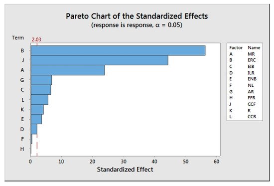
Figure 6. Pareto diagram of the system’s variables.
As represented in Figure 6 and Figure 7, eight variables were identified for marking cars, greenhouse gas emission rate of each car, greenhouse gas emission rate of each industrial building, greenhouse gas emission rate of each non-industrial unit, as well as forestry, cleaning rate of per hectare of forest, raining, and air cleaning rate of rain, which were the major pollution system’s variables.
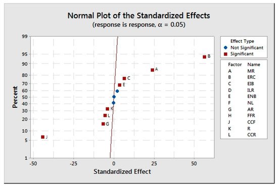
Figure 7. Normal diagram for identifying the major pollution variables.
Figure 8 indicates the optimized amount of each variable to reduce pollution.
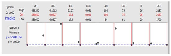
Figure 8. The optimal amount of each variable.