With the rapid development of artificial intelligence, big data, and data fusion technology, car driving tends to be intelligent and unmanned. Recently, research on Unmanned Ground Vehicles (UGVs) has become a hot topic at home and abroad ^[1][2][3][1,2,3]. Its core technologies include environmental awareness, vehicle positioning, path planning, and path tracking control ^[4][5][6][7][4,5,6,7]. Path tracking control, as a key core issue of unmanned driving technology, has attracted much attention from scholars and it ensures that the car drives on the specified path ^[7][8][9][7,8,9]. So, research on path tracking control has both theoretical and practical significance.

However, UGV path tracking control is a strongly nonlinear process, which contains time-varying characteristics, uncertainty, etc., and a precise mathematical model is difficult to obtain [10]. As artificial intelligence develops, neural networks can solve the above problem well due to their nonlinear approximation capabilities [11]. For example, a new end-to-end autonomous control method was proposed to simplify the separate modules in the traditional control pipeline into a single neural network [12]. A novel application of the biologically inspired computing paradigm was presented for solving the initial value problem (IVP) of electric circuits based on a nonlinear RL model by exploiting the competency of accurate modeling with a feed forward artificial neural network, the global search efficacy of genetic algorithms, and a rapid local search with sequential quadratic programming [13]. Moreover, predictive control, rooted in industrial engineering, is widely used. Usually, the schemes that combine a neural network model and predictive control are more popular and useful to solve the nonlinear control problem. For example, physics-based recurrent neural network modeling approaches were proposed for a general class of nonlinear dynamic process systems to improve the prediction accuracy by incorporating a priori process knowledge, and the proposed physics-based RNN models were utilized in model predictive controllers [14]. A neural-network-based technique for developing nonlinear dynamic models from empirical data for a model predictive control (MPC) algorithm was presented [15]. However, for the neural networks, they easily reach the local minimum [16].

2. System Description of the SUGV

A simplified SUGV model is shown in Figure 1. Two front wheels and two rear wheels are combined into a single front wheel and rear wheel, which are simplified into a two-degrees-of-freedom vehicle model. The following assumptions were made: we ignored the effect of steering and suspension; we kept the vehicle’s longitudinal speed constant and only considered the lateral movement along the y axis and the yaw movement around the z axis; we ignored the effects of horizontal and vertical aerodynamics; and we considered the side characteristics of the tire in the analysis of the tire force ^[17][18][19][36,37,38].

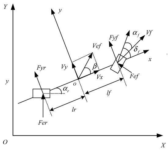
Figure 1. The SUGV model.

The XOY coordinate system in Figure 1 is a fixed geodetic coordinate system, and xoy is the structure of the coordinate system, which changes with the movement of the body. The force analysis of the above model along the y axis and around the z axis is obtained.

$$\{\begin{array}{l}M{a}_y=F_{cf\begin{array}{l}{}_{}\cos {\delta }_f+F_{cr\begin{array}{l}{}_{}\\ I_z\dot{w}=I_f{F}_{cf\begin{array}{l}{}_{}\cos {\delta }_f-I_r{F}_{cr\begin{array}{l}{}_{}\end{array}}\end{array}}\end{array}}\end{array}}\end{array}$$

(1)

where M is the vehicle’s weight; If is the distance between the center of the front axle and the center of mass of the vehicle; Ir is the distance between the center of the rear axle and the center of mass of the vehicle; Iz is the moment of inertia of the vehicle around the z axis; δf is the front wheel angle of the vehicle; w is the yaw velocity of the vehicle; and ay is the accelerated velocity of the vehicle along the y axis based on the xoy coordinate system, which mainly consists of the movement along the y axis and the centripetal acceleration Vxw. We can obtain:

$$a_y=\ddot{y}+V_{x}w$$

(2)

where Fcf and Fcr are the lateral force of the tire applied to the front and rear wheels of the vehicle, respectively. From the defined dynamic model, we can see that the side characteristic of the tire is considered in the analysis of the tire force. When the front wheel angle δf and the sideslip angle β are small, the sideslip characteristic of the tire is in a linear range. So, we can obtain

$$F_{cf{}_{}=2C_f{\alpha }_f}$$

(3)

$$F_{rf{}_{}=2C_r{\alpha }_r}$$

(4)

where Cf and Cr are the cornering stiffnesses of the front and rear tires, respectively. Since there are two front and rear wheels, the force is twice that of a single tire. αf and αr are the tire sideslip angle and the angle between the direction of the tire velocity vector and the x axis, respectively. At a small angle, the size of the two angles can be approximately expressed as:

$$$$ tan α f ≈ θ < V f ,   x > = V y + l f φ ˙ V x tanαf≈θ<Vf, x>=Vy+lfφ˙Vx

(5)

$$$$ tan α r ≈ θ < V r ,   x > = V y − l r φ ˙ V x tanαr≈θ<Vr, x>=Vy+lrφ˙Vx

(6)

According to the coordinate system relationship, the side slip angle is β=tanβ=VyVx. From (1)–(6), the differential equation of the vehicle dynamics model is obtained.

$$$$ { w ˙ = l f 2 C f + l r 2 C r I z v x w − l f C f + l r C r I z β + l f C f I z δ f β ˙ = ( − l f C f + l r C r m v x 2 − 1 ) w − C f + C r m v x β + C f m v x δ f ⎧⎩⎨⎪⎪⎪⎪w˙=l2fCf+l2rCrIzvxw−lfCf+lrCrIzβ+lfCfIzδfβ˙=(−lfCf+lrCrmv2x−1)w−Cf+Crmvxβ+Cfmvxδf

(7)

The control input and output variables of the controlled vehicle are the front wheel steering angle δf and the yaw velocity w, respectively. According to the vehicle dynamics model, a relation between the output and the input of the controlled system is deduced

$$$$ w ¨ ( t ) = − a 1 w ˙ ( t ) − a 2 w ( t ) + b 1 δ ˙ f ( t ) + b 2 δ f ( t ) w¨(t)=−a1w˙(t)−a2w(t)+b1δ˙f(t)+b2δf(t)

(8)

where $$ a 1 = m ( l f 2 C f + l r 2 C r ) + I z ( C f + C r ) m v x I z  a1=m(l2fCf+l2rCr)+Iz(Cf+Cr)mvxIz, a2=−mv2x(lfCf−lrCr)+CfCrmv2xIz, b1=lfCfIz, b2=CfCrLmvxIz. $$ a 2 = − m v x 2 ( l f C f − l r C r ) + C f C r m v x 2 I z . $$ b 1 = l f C f I z . $$ b 2 = C f C r L m v x I z .

So, the vehicle control system can be described as the following second-order system:

$$$$ { x ˙ 1 = x 2 x ˙ 2 = F ( x 1 , x 2 , δ ˙ f , γ ( t ) ) + b 0 δ f y = x 1 ⎧⎩⎨⎪⎪x˙1=x2x˙2=F(x1,x2,δ˙f,γ(t))+b0δfy=x1

(9)

where x1=w(t), x2=w˙(t), b0=b2, F(x1,x2,δ˙f,γ(t))=−a1w˙(t)−a2w(t)+b1δ˙f(t)+γ(t), and F(⋅) is defined as a generalized disturbance that includes the modeled and unmodeled parts of the vehicle and an unknown external disturbance.

3.2. Multi-Dimensional Taylor Network Model

If the function is m^+1-order differentiable everywhere in the neighborhood at some point, the power series of the eigenfunction expansion at this point is not greater than m^ power in terms of the principle of the multivariate Taylor formula. Based on the MTN model, as shown in Figure 2, the general dynamic equation of an t^-dimensional system can be expressed as ^[20][17]:

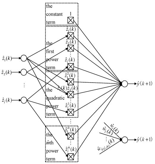
$$$$ y ^ ( k + 1 ) = ∑ p ^ = 1 N ^ ( t ^ , m ^ ) w ^ p ^ ( k ) ∏ q ^ = 1 t ^ z ^ q ^ λ ^ ( p ^ , q ^ ) ( k ) y^(k+1)=∑p^=1N^(t^,m^)w^p^(k)∏q^=1t^z^λ^(p^,q^)q^(k)

(10)

Figure 2. Diagram of the MTN.

In (10), N^(t^,m^) represents the total number of product items of the t^-ary function ο^[⋅], which is expanded into the approximate polynomial with m^ powers; w^p^(k) represents the weight coefficient of the p^-th product item in the formula; λ^(p^,q^) represents the power of the variable z^q^(k) in the p^-th product item; and ∑q^=1t^λ^(p^,q^)≤m^, where p^=1,2,⋯,N^(t^,m^).

As can be seen from Figure 2, the MTN is composed of three main layers, including the input layer, the middle layer, and the output layer. Its structure is simple, it contains only addition and multiplication operations, it is equivalent to only one neuron of the neural network, and it has low algorithm complexity, namely real-time performance. Otherwise, the model parameters are obtained through continuous optimization, which has a "self-learning" ability and good robustness.

The MTN model has a powerful approximation capability for nonlinear systems and can approximate any model with sufficient precision as long as N^(t^,m^) is large enough ^[21][22][21,39].