Voxelisation Algorithms: Comparison
Please note this is a comparison between Version 2 by Vicky Zhou and Version 3 by Vicky Zhou.

Voxel-based data structures, algorithms, frameworks, and interfaces have been used in computer graphics and many other applications for decades. There is a general necessity to seek adequate digital representations, such as voxels, that would secure unified data structures, multi-resolution options, robust validation procedures and flexible algorithms for different 3D tasks.

  • voxel
  • voxelisation
  • algorithms
  • geometric primitives

1. Introduction

Voxel-based representations are used in many application domains. In computer graphics, voxels are used for fast ray tracing [1], voxelisation of surfaces and solids [2][3], shadow [4] and visibility analysis [5][6][7]. These are mostly focused on fast-real time visualisation and therefore aiming at visualising only visible voxels. In medicine, voxel representations are commonly implemented in software processing CT and MRI scans investigating organs and body structure in three dimensions [8][9]. Voxel approaches are increasingly being used in city modelling for 3D reconstruction [10] and spatial analysis [11]. Voxel-based models are commonly investigated with the aim to define geological phenomena [12][13]. In environmental analysis, voxelisation is used to establish computational domains for gaseous and liquid simulations as well as to interact with obstacles [14]. Voxel-based methods are extensively applied for the processing of point clouds [15][16][17]. A quick voxelisation is suggested to derive navigable areas for pedestrian simulation [18][19][20] and collision detection [21][22]. As we can see voxels are highly applicable in various domains due to their discrete representation creating a continuous phenomenon in space.
A discrete approximation of digital objects or continuous phenomena is called voxelisation. Many different voxelisations are performed targeting lines [23], triangles [24], polygons [25], surfaces [26] and solids [2][3]. When voxelising 3D objects different properties can be considered such as connectivity, separation, coverage and tunnelling [27], as well as colours preservation [28] and anti-aliasing [29] which are related to non-binary voxelisation. Based on our knowledge there is no single paper that evaluates and presents the characteristics of available algorithms for the voxelisation of different geometrical primitives.
To be able to work with voxels, the conversion from vector-based primitives such as points, lines, triangles, surfaces and solids needs to be performed.

2. Voxelisation Properties

The literature provides many definitions of a voxel space. Here we will refer to a voxels space as to an integer space. A grid point represents a cell commonly referred to as a voxel. Voxels can have multiple properties, which can be organised differently with respect to the application. Binary voxelisation is a term to indicate that a voxel can have a property, which can take only two values: 0 (empty) or 1 (filled).

2.1. Common Voxelisation Properties

The shape of a voxel is generally considered as a cube, although applications may use cuboid representations [13]. The neighbourhood properties of a voxel play an important role in all voxel-based algorithms. A voxel can have a maximum of 26 adjacent voxels, from which 6 share a face, 12 share an edge and 8 voxels share only a corner in 3D space (Figure 1). Based on this, the adjacency relation N between two voxels is defined. Face-sharing voxels have adjacency 6, face-sharing and edge-sharing voxels have the adjacency of 18, and 26-adjacent voxels are those that share a face, edge or corner. Sensors 21 08241 g001
Figure 1. The 26 neighbours of a voxel; six voxels sharing face (in red), 12 voxels sharing edge (in green) and 8 voxels sharing a vertex (in blue).
In contrast to vector representations, voxelised objects are prone to several configurations such as holes, cavities and penetration, which have to be taken care of during the voxelisation. The objects have to remain connected so that a discrete unit represents correctly the analogous representation of the vector object. This implies that the voxelisation algorithms should apply several topological constraints such as connectivity, separation, coverage and tunnelling [27].
Connectivity identifies a set of N-paths between every pair of voxels belonging to an object and measures the way voxels are linked to each other. It gives a notion of ‘thin’ or ‘thick’ voxelisation.  Strongly connected voxels, such as 8-connected in 2D and 18 and 26-connected in 3D are very attractive since they result in tinner objects with shorter length or area, and require less memory for their storage. In some cases, the connectivity of voxels might be insufficient to estimate the quality of the voxelisation process and therefore the notion of separation needs to be investigated.
Separation is a set of N-path voxels that divides two sets of voxels. This notion is intended to present how the “empty space” interacts with the voxelised object. The separation is exclusively a topological property, which does not reflect to what extent the actual object is correctly represented. In 2D space, a 4-connecting voxelised object is always 8-separating and vice-versa (Figure 2). Separation is one of the main aspects that is considered in simulations preventing fluids to go through obstacles such as wall. In the case of 6-separating voxelisation (i.e., thin voxelisation) a fluid would be allowed to go to voxels that only share a face with a voxel. In general, such a kind of voxelisation is sufficient since fluids cannot travel to other voxels that share an edge or a corner with the central one. In favour of having 6-separating voxelisation is the fact that it is cheaper to compute and often more required in computer graphic applications [30].
Sensors 21 08241 g002
Figure 2. Connectivity and separation in 2D voxel set representing a circle. On the left, 4-connected voxelisation is achieved, which is at the same time 8-separating. On the right, 8-connected, and thus, 4-separating voxelisation is presented.
Coverage is a notion that aims to define formally the thickness of a voxelised line or surface. There are three major variations of it: cover, supercover and partial cover (Figure 3). A set of voxels is called a cover if every point of an object is in a voxel. Normally, 8-connectivity in 2D creates a cover. A set of voxels are called supercover if all voxels that ‘contain’ or ‘touch’ points of the object are included in the set. In general, it enlarges the object and may result in large overlapping parts of neighbouring objects [23]. A suvercover is also known as a conservative voxelisation [37,38], which is highly desirable for applications such as collision detection, occlusion culling and visibility analysis. A partial cover is a subset of cover, which allows for the maintenance of the tiniest voxelisation. Another approach solution can target a ‘well-voxelised’ approximation, which is tunnel-free and has a partial cover at the same time. To achieve such voxelisation, a method is proposed where the Euclidian distance is minimal between centroids of voxels representing a cover and the continuous object [27]. Sensors 21 08241 g003
Figure 3. Representation of a cover (a), supercover (b), partial cover (c), and partial cover (d) well-voxelised curve in 2D.
Tunnelling is the notion to indicate the effect of penetration of two voxelised lines or surfaces. The 8-connected voxelisation in 2D, and 18- and 26-connected in 3D are prone to tunnelling. Consequently, a 4-connected voxel path in 2D and 6-connected in 3D are tunnel-free. In computer graphics, tunnelling may give the impression of having holes during rendering [23]. In applications performing analysis on voxelised objects, tunnelling might lead to difficulties in detecting intersections and penetrations.

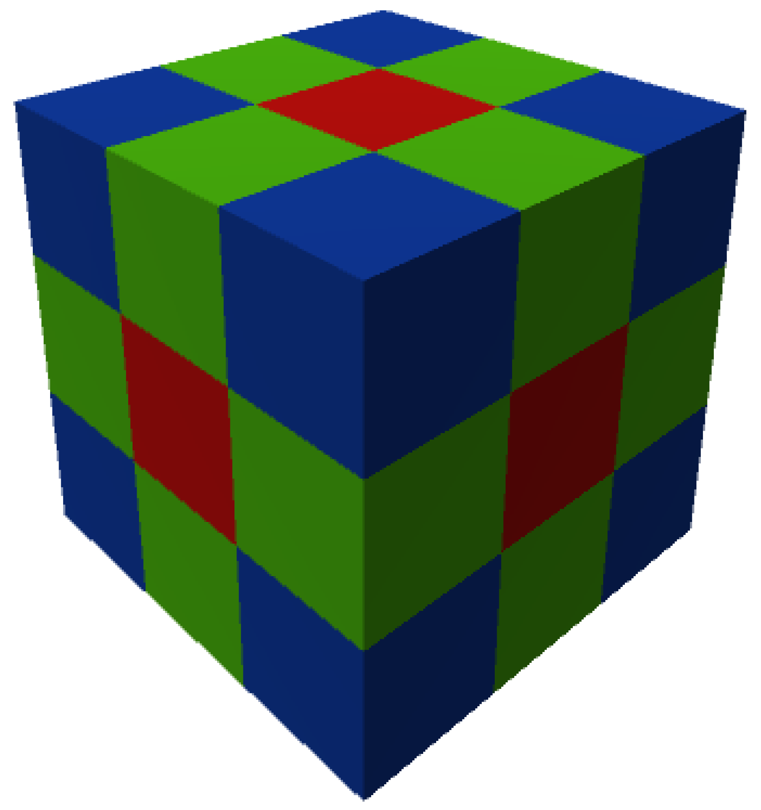
2.2. Binary and Non-Binary Voxelisation

A common voxelisation classification depending on the resulting output identifies two types of voxelisation: binary and non-binary. Binary voxelisation is investigated by many researchers [3][31][32][33], but we need to explain the needs and possibilities of using non-binary voxelisation.
The main advantages of using binary voxelisation over a non-binary one is memory requirements, where only a single bit is needed to indicate a voxel’s status, and speed to create a voxelised object. Apart from a discrete representation of an object that binary representation provides, many times storing additional information is needed, especially for objects that come with textures, semantics and other properties. For example, we can store information related to surface normal and material properties like colour, opacity, density, depth, etc. There are several classes of non-binary voxelisation targeting anti-aliasing [29][34], multi values [35][36][37][38], and distance transform [39][40][41][42].

3. Voxelisation of Geometric Primitives

Many voxelisation approaches have been reported in the literature, for example: for lines [23], triangles [24], polygons [25], parametric surfaces [34], implicit surfaces [43], constructive solid geometry [44], and polyhedral objects [45], etc. Herein will present the state-of-the-art methods for voxelisation of geometric primitives such as points, lines, triangles, surfaces and solids.

3.1. Point Voxelisation

Voxelisation of a point or many points can be done in a very straightforward way considering a pivot point of grid space and voxel size. An algorithm considering the integer values for centroids of voxels is presented in [46]. Due to its simplicity to calculate and the ability to run in parallel, a point voxelisation technique known as particle-in-cell (PIC) is used in physical simulations to track the movement of densities and currents in voxel space [47].

3.2. Line Voxelisation

A 3D continuous line can be transformed into a discrete set of connected voxels, and used as a building block for generating more complex 3D objects, ray traversal in voxel space [23], and voxelisation of more complex primitives like triangles [33]. In 3D, 6-connected and 26-connected line voxelisation techniques are usually discussed by researchers. Since not all line are straight spline voxelisaion is explored as well.

3.2.1. 6-Connected Voxelisation Algorithms

A straightforward method of raymarching voxels in a uniform grid was proposed generating a 6-connected path, which is nowadays known as the real line voxelisation (RLV) [1]. The method traverses the intersections between a line and the grid. If the line passes through the corner of the voxel grid, an arbitrary voxel candidate can be picked or supercover line voxelisation (SLV) can be formed.
Another algorithm producing 6-connected voxelisation is Xiaolin Wu’s line algorithm [48]. This algorithm is commonly used in modern computer graphics because it supports antialiasing while being fast compared to other available algorithms.

A method generating a 6-connected line, named tripod, is proposed suggesting a comparable performance in voxelisation speed with the RLV algorithm [23]. The method is tracking the projections of a line on the three main axes. However, it requires the line of origin to lay at the centre of the voxel to avoid fractions in calculations, which might not achieve the containment of the original line (Figure 4c).

Following the same structure as RLV, a new approach is presented called integer-only line voxelisation (ILV) [41]. The main idea of this method is to avoid floating-point arithmetic and divisions present in RLV. Apart from the shift of the starting point of a line as in the tripod algorithm, this algorithm shifts the endpoint to the voxel centre as well (Figure 4d).

Sensors 21 08241 g005

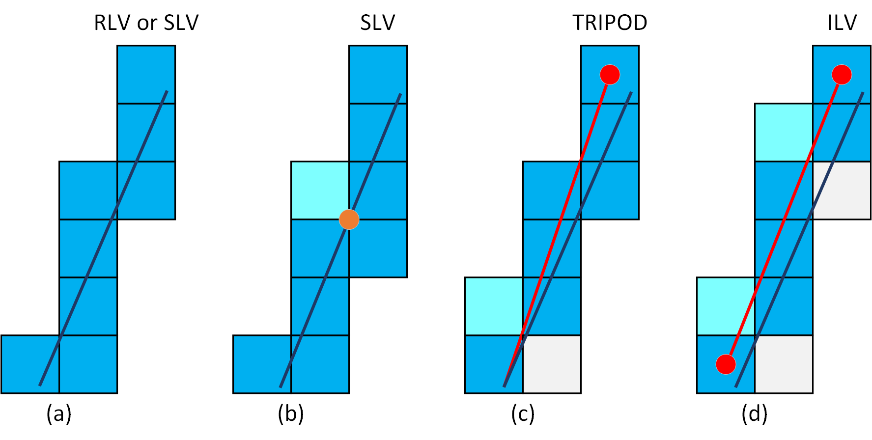
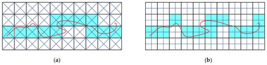
Figure 4. (a) RLV or SLV; (b) SLV generates more voxels than RLV considering all touching voxels; (c,d) small variations of the voxels coverage generated by Tripod and ILV algorithm.

3.2.2. 26-Connected Voxelisation Algorithms

Many algorithms create thin line voxelisation. Regarding 8-connected rasterisation, the most famous algorithms are digital differential analyser (DDA) (https://en.wikipedia.org/wiki/Digital_differential_analyzer_(graphics_algorithm). (accessed on 30 December 2021)) and Bresenham’s line algorithm [49]. The main difference between these two algorithms is that Bresenham’s line algorithm employs integer with round off functions while the DDA algorithm works with floating-point values. Another pro of using Bresenham’s algorithm is the computational performance mainly due to using additions and subtractions compared to the DDA which uses multiplications and additions. Unlike the DDA algorithm, the Bresenham algorithm is an integer-only line voxelisation algorithm, requiring endpoints to lie exactly on the middle points of the grid. However, we should point out that this shift can result in the coverage of different voxels between these two algorithms. A 3D version of DDA [50] and Bresenham’s algorithm [51] are also proposed creating a 26-connected line, behaving in the same way as the initial algorithms.

3.2.3. Spline Voxelisation Algorithms

To tackle a variety of lines, including parametric ones, Laine introduced two approaches considering intersections between specific targets and the grid [52]. Targets that are suggested are diagonal and crosshair ones. The targets can be applied in 2D and 3D voxelisations. Using one of these intersecting targets results in a voxelisation with different connectivity and separability properties. Generally, a diagonal target leads to 4-connectivity and a crosshair target to 8-connectivity voxelisation in 2D (Figure 5). The process is performed for each voxel which can be optimised by casting rays diagonally and horizontally from two directions for both scenarios in 2D or by intersecting planes in the same way for 3D. Another possible solution that we can think of is to approximate such a line with straight lines and use some of the previously mentioned algorithms to voxelise them.
Figure 5. Voxelisation of a curve using intersecting targets in 2D. (a) Using cross-diagonal intersection targets forming 4-connected and 8-separating voxelisation. (b) Using crosshairs intersection targets forming 8-connected and 4-separating voxelisation.

3.2.4. Comparison of Line Voxelisation Algorithms

When it comes to speed, integer-based algorithms achieving thinner voxelisation should be the quickest. However, this can depend on the application in which they are used. Thus, targeting optimal scanline voxelisation of 3D models RLV outperformed the 3D Bresenham’s line algorithm and ILV in terms of speed and accuracy of approximating original 3D models [53]. It is pointed out that the main reason for this is the consideration of many edge cases, in which case other algorithms were slower. Tripod and 3D-DDA were not considered here.
Table 1. Line voxelisation algorithms.
Method Type Property General Purpose
2D Bresenham’s line algorithm [49] Integer-only 8-connected Line primitives rasterisation
2D-DDA Floating-point or integer 8-connected Line primitives rasterisation
3D-DDA [50]
[Floating-point or integer 226-connected Line primitives voxelisation
] Slice-based RLV & SLV [1] Floating-point Conservative Line primitives voxelisation
Xiaolin Wu’s line algorithm [48]
] and midpoint traversal [62] are available. Tiled traversal algorithms are considered the best out of them. However, this might not be the case if triangles are smaller compared to a selected pixel size [63], requiring to split them into groups for faster processing [26].
It is suggested that DDA and Bresenham algorithms can be used for triangle rasterisation, but they can be difficult to implement in hardware resulting in a few approaches relying on them for triangle voxelisation [62]. However, researchers are trying to come up with approaches that actually involve line rasterisation [33][53], achieving compareble preformance with above mentioned approaches.

3.3.2. Raycasting

Several algorithms are targeting ray-triangle intersections to derive which triangles to render on a screen [64][65]. Ray casting can be performed from a specific point of view using a perspective camera or an orthogonal camera, where rays are uniformly sent towards an area of interest. However, voxels do not cover the same area in the scene if a perspective camera is used. On the other hand, if all intersections with triangles are identified using an orthogonal camera, the whole scene can be voxelised at once with the same size voxels. In order not to miss thin structures, raycasting can be performed in all three directions or diagonally. To reduce the intersection checks between triangles and rays an algorithm is proposed which checks first if bounding boxes of triangles are inside the view frustum [66].
Similar techniques are used for the efficient calculation of ray-polygon intersections. For convex polygons dividing them into triangles and performing inside-outside check is suggested [67], while for non-convex and self-intersecting polygons odd/even parity can be used for a ray-polygon intersection [68]. Another set of algorithms achieving 6-connected and 26-connected voxelisation are presented [46], which are based on the previously mentioned targets intersections.

3.3.3. Comparison of Triangle Voxelisation Algorithms

Rasterisation techniques are predominantly used for voxelisation of triangles (Table 2). Although ray casting techniques are slower than rasterisation ones, they can be used at the same time to obtain shadows and reflections more accurately for computer graphics applications. Raycasting techniques can achieve 6- and 26-connected voxelisation, while conservative voxelisation can be only achieved with rasterisation techniques.
Table 2. Triangle voxelisation algorithms.
Rendering
[14] Slice-based ‘26-connected’ Depth peeling Rendering
[70] Slice-based Conservative Bounding box Collision detection
Interior only Bitwise OR operation Rendering [63] Rasterisation 26-connected
[Bounding box 28Rendering ] Slice-based Interior only Mask creation Voxelisation Floating-point Conservative Antialiasing
[31] Tripod [23] Integer 6-connected Line primitives voxelisation
3D Bresenham’s line algorithm [51] Integer-only 26-connected Line primitives voxelisation
Targets-based approaches [52] Floating-point 6/26-connected Irregular line primitives voxelisation
ILV [33] Integer-only 6-connected Surface voxelisation

3.3. Triangle Voxelisation

Triangles are the most basic polygons which have some unique properties such as being planar, having a well-defined interior and can perform quick intersections with rays. Triangles are almost always used as a building element of more complex objects like polygons and surfaces. In general, rasterisation is the main technique used for voxelisation of triangles, but raycasting techniques can be used as well (Figure 6).
Sensors 21 08241 g007
Figure 6. Triangle voxelisation. (a) uniform ray casting (b) rasterisation techniques; in red, the bounding box, in green tiles that are outside; in purple tiles that are inside; in yellow tiles that are intersecting the triangle are presented.

3.3.1. Rasterisation

Rasterisation approaches mainly rely on bringing triangles into 2D space to identify quickly which pixels should be filled using inside/outside checks. To optimise which pixels to check, as presented in Figure 6b, the simplest approach is to consider only pixels that are covered by the bounding box of a triangle [54]. However, for elongated triangles, many pixels that are outside still need testing, which can be considered as wasted computation. As a result, an approach tessellating a bounding box space into tiles is proposed (Figure 6b), which can quickly eliminate large blocks of pixels that are outside but also inside of a triangle [55]. At the same time, many rasterisation approaches target various pixel traversal ways to quickly identify which to fill. Thus, algorithms considering backtrack traversal [56], zigzag traversal [57], central-line traversal [54][58], tiled traversal [59][60][61
[
71
]
Rasterisation 26-connected Bounding box Rendering
Slice-based Interior only & conservative Single pass & bitwise OR operation Voxelisation [73] Rasterisation 26-connected Tile-based Voxelisation
[3] Rasterisation Interior only Tile-based, bounding box, sparse octree Voxelisation & storage [3] Rasterisation Conservative & 26-connected Bounding box Voxelisation
[75] Rasterisation ‘Conservative’ Two level grids Rendering
[26] Rasterisation Conservative & 26-connected Tile-based & bucketing Voxelisation & rendering
[32] Rasterisation 26-connected Point tessellation Voxelisation
[46] Raycasting 6/26-connected Intersecting targets Voxelisation
[33] Rasterisation 6/26-connected ILV Voxelisation
[37] Rasterisation & raycasting Conservative Tile-based + ray-triangle intersection Voxelisation & rendering
Method Type Property Main Technique
[3][54][56][57][58][62] Rasterisation 6/26-connected & conservative Bounding box, backtrack, zigzag, central-line, and midpoint traversal
[3][26][59][60][61] Rasterisation 6/26-connected & conservative Tile-based
[46][64][65][66][68] Raycasting 6/26-connected Ray-triangle and ray-polygon intersection
[33][53] Rasterisation 6/26-connected & conservative Line rasterisation

3.4. Surface Voxelisation

A surface usually represents a continuous object resembling a deformed plane. To achieve a surface voxelisation there are two main approaches. The first approach is based on slicing of a scene or an object from one or more viewing directions. The second one considers rasterisation of triangles in 2D based on the dominant axis and the identification of overlapping voxels in 3D space. Another known classification divides approaches using graphics pipeline and computational voxelisation [69].

3.4.1. Slice-Based

Regarding slice-based voxelisation, several algorithms are proposed [14][35]. ]. The main idea behind this approach is to perform voxelisation from a viewpoint slice-wise. However, it can miss thin structures (e.g., trees branches) and have discontinuity between voxels, especially in the case of considering one viewing direction [3]. To capture all pixels overlapped by triangles and then identity for each pixel depth range along the viewing direction, conservative voxelisation is proposed [70]. This can definitely address the issues, but some additional voxels may be set in the depth range computation due to robustness problems [3].

3.4.2. Rasterisation

Many approaches perform triangle rasterisation obtaining a voxelised model. Some of them use bounding boxes of triangles to test which voxels to cover [3][63][71], while others rely on a tile-based voxelisation [26][72][73] where triangles are assigned to each tile they overlap.
Using a triangle/box overlapping technique it is possible to assign one thread per triangle and test each pixel for coverage. This approach relies on a 2D axis-aligned box to test coverage. Tile-based approaches as discussed previously can boost voxelisation performance since not all pixels will be tested. Both approaches are suitable for running the voxelisation in parallel to achieve fast performance [3][26]. However, there can be a huge overhead if models are represented by small triangles compared to a selected pixel size [74]. To mitigate this issue Pantaleoni introduced coarse and fine rasterisation, where tiles are split based on the number of triangles during the coarse rasterisation for better load balancing in the fine rasterisation step afterwards. A similar approach was presented by Kalojanov [75] concentrating more on fast rendering, keeping all overlapping triangles per voxel, where conservative voxelisation was not strictly identified. Another approach using point-tessellated voxelisation is proposed afterwards [32]. The method calculates a triangle tessellation factor to subdivide triangles into micro triangles, in which centroids are voxelised afterwards to obtain a voxelised model. However, this approach can miss voxelising some voxels and it is not necessarily quicker. Recent work uses line voxelisation at its core to identify filled voxels for each triangle of a surface model [33]. By using either SLV or ILV approach a suvercover or 26-tunnel-free surface voxelisation can be identified. The method can downgrade the voxelisation to generate tinner surfaces like 18- or 6-tunnel-free ones. A hybrid approach relying on tile-based rasterisation and raycasting is also proposed for effective rendering of surface and solid voxelisation [37].

3.4.3. Comparison of Surface Voxelisation Algorithms

Table 3 shows the most recent methods used to achieve fast surface voxelisation, where most of them use rasterisation to identify a voxel representation. Some of the methods are more flexible and can achieve with small modifications different voxelisation properties, whereas others are more specific. It is hard to tell which method is the most robust, but possibly the methods by Pantaleoni [26] and Zhang [33] can be suggested as the best. In comparison, the method presented by Zhang outperformed the ones presented by Pantaleoni, where the ILV method generated slightly more voxels. However, it is pointed out by the authors that additional information (colour, surface normal vectors, and so on) cannot be stored during voxelisation, which is not the case with Pantaleoni’s approaches.
Table 3. Surface voxelisation algorithms.
Method Type Property Main Technique General Purpose
[35] Slice-based ‘26-connected’ Plane slicing

3.5. Solid Voxelisation

As opposed to voxels covering a shell (i.e., surface) of an object, in a solid voxelisation, voxels whose centroids are inside the object are taken into account. Sometimes a boundary representing the surface of a solid object can be voxelised as well [35]. Methods utilised to acquire solid voxelisation are similar to the surface ones, considering either rasterisation [3] or slicing [2][28][31][35][76]. Solid voxelisation can be used for translucency effects, volume visualisations used to show CT scans, particle collision detection and interaction, morphological operations, and CSG operations [31]. By counting the number of voxels representing an object, volume can be calculated [77], which can be identified even more accurately if object-voxel coverage factor is recorded [3].
It should point out that all current approaches are concentrating on solid voxelisation of watertight models. In watertight models, all points of each connected component have a clear separation between the interior and exterior.

3.5.1. Slice-Based

A slice-based algorithm for solid voxelisation using a clipping plane to generate a 2D slice is proposed [35], where a logical XOR operation between the previous and current slices are used to achieve a solid voxelisation. However, only a binary voxelisation is generated due to XOR operations, and some voxels can be missed. An approach relying on surface voxelisation and consequent 2D scan-filling in all three directions is proposed [76]. This approach suggests encoding binary voxels in separate bits of multiple targets, enabling processing many slices in a single pass. However, the algorithm fails if two fragments are located in the same voxel. An algorithm achieving multi-valued solid voxelisation is suggested using depth buffer and stencil buffer to create a mask for solid slice creation [28]. Building on top of their previous research [2], an approach for solid voxelisation is presented where all slices are processed at a time using more robust bitwise OR operation [31]. The authors also presented how to achieve solid conservative voxelisation, combining their solid voxelisation and conservative surface voxelisation of Zhang [70].

3.5.2. Rasterisation

Two types of triangles-based solid voxelisation are presented [3]. The first one is based on rasterisation of each triangle considering their bounding boxes, while the other one assigns triangles into tiles to speed up the voxelisation process for situations when the grid size is large, or the model contains many triangles. For both approaches, flipping the voxels in one direction is necessary to achieve solid voxelisation. The authors proposed one more approach which uses sparse octree performing first slightly modified conservative surface voxelisation to identify active voxels that will be stored in an octree, followed by hierarchical inside/outside propagation to achieve solid voxelisation. This approach is slower than the other two, whereas it requires less memory and enables direct rendering into a sparse spatial data structure.

3.5.3. Comparison of Solid Voxelisation Algorithms

Table 4 shows the most recent approaches used for solid voxelisation, where the approaches by Schwarz and Seidel [3] and Eisemann and Décoret [31] represent state-of-the-art methods for solid voxelisation. In general, Schwarz and Seidel approaches outperformed the approach of Eisemann and Décoret for smaller grid sizes, while the former one was faster for more complex models. The inner part of objects is usually voxelised, but these methods can be relatively easily extended to obtain the surface’s voxels at the same time.
Table 4. Solid voxelisation algorithms.
Method Type Property Main Technique General Purpose
[35] Slice-based Interior only Plane slicing Voxelisation
[76] Slice-based Interior only Surface voxelisation + 2D scan-filling Voxelisation

4. Conclusions

We see that voxelisation is used in many areas, and it can be quite diverse in many aspects. In Section 2, we covered the main concepts considered in voxelisation such as connectivity, separability, coverage, as well as tunnel-freeness. We can say that 26-connected voxelisation usually requires less time and memory to be created and stored compared to 6-connected and conservative voxelisation. A 6-separated voxelisation is usually sufficient for applications such as fluid simulations. For collision detection, occlusion culling and visibility processing conservative voxelisation is highly desirable. Tunnelling can be addressed if 6-connected voxelised lines are used to send rays or to intersect with objects. The other option would be to consider either 6-connected or conservative voxelisation for all objects. The usage of binary and non-binary voxelisation is presented as well, indicating that non-binary voxelisation might be even more applicable than binary one.

Regarding 3D primitives, we examined voxelisation of points, lines, triangles, surfaces, and solids. In terms of line voxelisation, we split the algorithms into three groups, where the first two deal with different types of connectivity, while the third group focuses on voxelisation of curves. For triangles, we examined how rasterisation and raycasting techniques can be used. In terms of surfaces and solids, we identified that slice-based and rasterisation techniques are mainly used to perform voxelisation. We can see that surface voxelisation is investigated by the greatest number of researchers. There are several reasons for this. Firstly, surface voxelisation achieves smaller memory output and is faster compared to solid voxelisation. Secondly, some of the very common requirements such as collision detection, fluid simulations and ray tracing can be easily achieved based on them. We should point out that all algorithms for solid voxelisation concentrate on the voxelisation of watertight models, which is not necessarily sufficient for some application domains like building information modelling (BIM) where objects may have overlaps.

We presented here a vast number of algorithms targeting voxelisation of different geometric primitives. The greatest challenge is the availability of these algorithms for testing and further research, which usually requires building them from scratch in a possibly nonoptimal way. Therefore, creating a library with these algorithms would definitely facilitate the development of new approaches for voxelisations. Another interesting idea is to develop a database that would use some of the presented data structures to effectively store and process voxels.

References

  1. Amanatides, J.; Woo, A. A Fast Voxel Traversal Algorithm for Ray Tracing; Eurographic: Goslar, Germany, 1987; Volume 87, pp. 3–10.
  2. Eisemann, E.; Décoret, X. Fast scene voxelization and applications. In Proceedings of the 2006 Symposium on Interactive 3D Graphics and Games, Redwood City, CA, USA, 14–17 March 2006; pp. 71–78.
  3. Schwarz, M.; Seidel, H.-P. Fast parallel surface and solid voxelization on GPUs. ACM Trans. Graph. 2010, 29, 1–10.
  4. Gorte, B.G.H.; Zhou, K.; van der Sande, C.J.; Valk, C. A computationally cheap trick to determine shadow in a voxel model. ISPRS Ann. Photogramm. Remote Sens. Spat. Inf. Sci. 2018, 4, 67–71.
  5. Reinbothe, C.K.; Boubekeur, T.; Alexa, M. Hybrid Ambient Occlusion; Eurographics: Goslar, Germany, 2009; pp. 51–57.
  6. Nichols, G.; Penmatsa, R.; Wyman, C. Interactive, multiresolution image-space rendering for dynamic area lighting. In Computer Graphics Forum; Blackwell Publishing Ltd.: Oxford, UK, 2010; Volume 29, pp. 1279–1288.
  7. Aleksandrov, M.; Zlatanova, S.; Kimmel, L.; Barton, J.; Gorte, B. Voxel-based visibility analysis for safety assessment of urban environments. In Proceedings of the ISPRS Annals of the Photogrammetry, Remote Sensing and Spatial Information Sciences, Singapore, 24–27 September 2019; Volume 4.
  8. Petoussi-Henss, N.; Zankl, M.; Fill, U.; Regulla, D. The GSF family of voxel phantoms. Phys. Med. Biol. 2001, 47, 89–106.
  9. Caon, M. Voxel-based computational models of real human anatomy: A review. Radiat. Environ. Biophys. 2004, 42, 229–235.
  10. Nießner, M.; Zollhöfer, M.; Izadi, S.; Stamminger, M. Real-time 3D reconstruction at scale using voxel hashing. ACM Trans. Graph. 2013, 32, 1–11.
  11. Beckhaus, S.; Wind, J.; Strothotte, T. Hardware-based voxelization for 3D spatial analysis. In Proceedings of the 5th International Conference on Computer Graphics and Imaging, Athens, Greece, 8–10 July 2002; Volume 20.
  12. Jørgensen, F.; Møller, R.R.; Nebel, L.; Jensen, N.-P.; Christiansen, A.V.; Sandersen, P.B.E. A method for cognitive 3D geological voxel modelling of AEM data. Bull. Eng. Geol. Environ. 2013, 72, 421–432.
  13. Stafleu, J.; Dubelaar, C.W. Product specification subsurface model GeoTOP. TNO Rep. 2016, R10133.
  14. Li, W.; Fan, Z.; Wei, X.; Kaufman, A. GPU-based flow simulation with complex boundaries. GPU Gems 2003, 2, 747–764.
  15. Huang, M.; Wei, P.; Liu, X. An efficient encoding voxel-based segmentation (EVBS) algorithm based on fast adjacent voxel search for point cloud plane segmentation. Remote Sens. 2019, 11, 2727.
  16. Poux, F.; Billen, R. Voxel-based 3D point cloud semantic segmentation: Unsupervised geometric and relationship featuring vs deep learning methods. ISPRS Int. J. Geo-Inf. 2019, 8, 213.
  17. Vo, A.-V.; Truong-Hong, L.; Laefer, D.F.; Bertolotto, M. Octree-based region growing for point cloud segmentation. ISPRS J. Photogramm. Remote Sens. 2015, 104, 88–100.
  18. Kyaw, A.S. Unity 4. X Game AI Programming; Packt Publishing Ltd.: Birmingham, UK, 2013.
  19. Gorte, B.; Aleksandrov, M.; Zlatanova, S. Towards egress modelling in voxel building models. ISPRS annals of the photogrammetry, remote sensing and spatial information sciences. In Proceedings of the 4th International Conference on Smart Data and Smart Cities, Kuala Lumpur, Malaysia, 1–3 October 2019; Volume 4.
  20. Gorte, B.; Zlatanova, S.; Fadli, F. Navigation in indoor voxel models. ISPRS Ann. Photogramm. Remote Sens. Spat. Inf. Sci. 2019, 4, 279–283.
  21. Boyles, M.; Fang, S. Slicing-based volumetric collision detection. J. Graph. Tools 1999, 4, 23–32.
  22. Silver, D.; Gagvani, N. Shape-based volumetric collision detection. In Proceedings of the 2000 IEEE Symposium on Volume Visualization (VV 2000), Salt Lake City, UT, USA, 9–10 October 2000; pp. 57–61.
  23. Cohen-Or, D.; Kaufman, A. 3D line voxelization and connectivity control. IEEE Comput. Graph. Appl. 1997, 17, 80–87.
  24. Dachille, F., IX; Kaufman, A. Incremental triangle voxelization. In Proceedings of the Graphics Interface, Montreal, QC, Canada, 15–17 May 2000; pp. 205–212.
  25. Kaufman, A.; Shimony, E. 3D scan-conversion algorithms for voxel-based graphics. In Proceedings of the 1986 workshop on Interactive 3D graphics, New York, NY, USA, 1 January 1987; pp. 45–75.
  26. Pantaleoni, J. VoxelPipe: A programmable pipeline for 3D voxelization. In Proceedings of the ACM SIGGRAPH Symposium on High Performance Graphics, Vancouver, BC, Canada, 5–7 August 2011; pp. 99–106.
  27. Cohen-Or, D.; Kaufman, A. Fundamentals of surface voxelization. Graph. Model. Image Process. 1995, 57, 453–461.
  28. Liao, D. GPU-accelerated multi-valued solid voxelization by slice functions in real time. In Proceedings of the 24th Spring Conference on Computer Graphics, Budmerice, Slovakia, 21–23 April 2008; pp. 113–120.
  29. Wang, S.W.; Kaufman, A.E. Volume sampled voxelization of geometric primitives. In Proceedings Visualization’93, San Jose, CA, USA, 25–29 October 1993; IEEE: New York, NY, USA, 1999; pp. 78–84.
  30. Crassin, C.; Green, S. Octree-based sparse voxelization using the GPU hardware rasterizer. OpenGL Insights 2012, 303–318. Available online: https://research.nvidia.com/publication/octree-based-sparse-voxelization-using-gpu-hardware-rasterizer (accessed on 30 November 2021).
  31. Eisemann, E.; Décoret, X. Single-pass gpu solid voxelization and applications. In Proceedings of the GI’08: Proceedings of the Graphics Interface, Windsor, ON, Canada, 28–30 May 2008.
  32. Fei, Y.; Wang, B.; Chen, J. Point-tessellated voxelization. In Proceedings of the Graphics Interface 2012, Toronto, ON, Canada, 28–30 May 2012; pp. 9–18.
  33. Zhang, Y.; Garcia, S.; Xu, W.; Shao, T.; Yang, Y. Efficient voxelization using projected optimal scanline. Graph. Models 2018, 100, 61–70.
  34. Sramek, M.; Kaufman, A.E. Alias-free voxelization of geometric objects. IEEE Trans. Vis. Comput. Graph. 1999, 5, 251–267.
  35. Fang, S.; Chen, H. Hardware accelerated voxelization. Comput. Graph. 2000, 24, 433–442.
  36. Heidelberger, B.; Teschner, M.; Gross, M.H. Volumetric collision detection for derformable objects. CS Tech. Rep. 2003, 395, 9.
  37. Young, G.; Krishnamurthy, A. GPU-accelerated generation and rendering of multi-level voxel representations of solid models. Comput. Graph. 2018, 75, 11–24.
  38. Zhang, Z.; Morishima, S.; Wang, C. Thickness-aware voxelization. Comput. Animat. Virtual Worlds 2018, 29, e1832.
  39. Sigg, C.; Peikert, R.; Gross, M. Signed distance transform using graphics hardware. In Proceedings of the IEEE Visualization, Seattle, WA, USA, 22–24 October 2003; IEEE: Manhattan, NY, USA, 2003; pp. 83–90.
  40. Varadhan, G.; Krishnan, S.; Kim, Y.J.; Diggavi, S.; Manocha, D. Efficient max-norm distance computation and reliable voxelization. In Symposium on Geometry Processing; ACM Digital Library: New York, NY, USA, 2003; pp. 116–126.
  41. Jones, M.W.; Baerentzen, J.A.; Sramek, M. 3D distance fields: A survey of techniques and applications. IEEE Trans. Vis. Comput. Graph. 2006, 12, 581–599.
  42. Novotny, P.; Dimitrov, L.I.; Sramek, M. Enhanced voxelization and representation of objects with sharp details in truncated distance fields. IEEE Trans. Vis. Comput. Graph. 2009, 16, 484–498.
  43. Stolte, N. Robust Voxelization of Surfaces; Center for Visual Computing and Computer Science Department, State University of New York at Stony Brook: Stony Brook, NY, USA, 1997; Available online: http://citeseerx.ist.psu.edu/viewdoc/download?doi=10.1.1.22.1047&rep=rep1&type=pdf (accessed on 30 November 2021).
  44. Liao, D.; Fang, S. Fast CSG voxelization by frame buffer pixel mapping. In Proceedings of the 2000 IEEE Symposium on Volume Visualization (VV 2000), Salt Lake City, UT, USA, 9–10 October 2000; IEEE: Manhattan, NY, USA, 2000; pp. 43–48.
  45. Gorte, B.; Zlatanova, S. Rasterization and Voxelization of Two- and Three-dimensional Space Partitionings. Int. Arch. Photogramm. Remote Sens. Spat. Inf. Sci. 2016, 41, 283–288.
  46. Nourian, P.; Gonçalves, R.; Zlatanova, S.; Ohori, K.A.; Vo, A.V. Voxelization Algorithms for Geospatial Applications: Computational Methods for Voxelating Spatial Datasets of 3D City Models Containing 3D Surface, Curve and Point Data Models. MethodsX 2016, 3, 69–86.
  47. Birdsall, C.K. Particle-in-cell charged-particle simulations, plus Monte Carlo collisions with neutral atoms, PIC-MCC. IEEE Trans. Plasma Sci. 1991, 19, 65–85.
  48. Wu, X. An efficient antialiasing technique. ACM Siggraph Comput. Graph. 1991, 25, 143–152.
  49. Bresenham, J.E. Algorithm for computer control of a digital plotter. IBM Syst. J. 1965, 4, 25–30.
  50. Fujimoto, A.; Tanaka, T.; Iwata, K. Arts: Accelerated ray-tracing system. IEEE Comput. Graph. Appl. 1986, 6, 16–26.
  51. Liu, X.W.; Cheng, K. Three-dimensional extension of Bresenham’s algorithm and its application in straight-line interpolation. Proc. Inst. Mech. Eng. Part B J. Eng. Manuf. 2002, 216, 459–463.
  52. Laine, S. A topological approach to voxelization. Comput. Graph. Forum 2013, 32, 77–86.
  53. Håkansson, T. A Comparison of Optimal Scanline Voxelization Algorithms. Master’s Thesis, Computer Science and Software Engineering, Linköping University, Linköping, Sweden, 2020.
  54. Pineda, J. A parallel algorithm for polygon rasterization. In Proceedings of the 15th Annual Conference on Computer Graphics and Interactive Techniques, New York, NY, USA, 1–5 August 1988; pp. 17–20.
  55. Akenine-Möller, T.; Aila, T. Conservative and tiled rasterization using a modified triangle set-up. J. Graph. Tools 2005, 10, 1–8.
  56. Woo, R.; Choi, S.; Sohn, J.-H.; Song, S.-J.; Bae, Y.-D.; Yoo, H.-J. A low-power 3D rendering engine with two texture units and 29-Mb embedded DRAM for 3G multimedia terminals. IEEE J. Solid-State Circuits 2004, 39, 1101–1109.
  57. Akenine-Möller, T.; Ström, J. Graphics for the masses: A hardware rasterization architecture for mobile phones. In ACM SIGGRAPH 2003 Papers; Association for Computing Machinery: New York, NY, USA, 2003; pp. 801–808.
  58. Ma, Y.; Wang, X.; Zhu, M.; Wan, W. Rasterization of geometric primitive in graphics based on FPGA. In Proceedings of the 2010 International Conference on Audio, Language and Image Processing, Shanghai, China, 23–25 November 2010; IEEE: Manhattan, NY, USA, 2010; pp. 1211–1216.
  59. McCormack, J.; McNamara, R. Tiled polygon traversal using half-plane edge functions. In Proceedings of the ACM SIGGRAPH/EUROGRAPHICS Workshop on Graphics Hardware, Interlaken, Switzerland, 21–22 August 2000; Association for Computing Machinery: New York, NY, USA, 2000; pp. 15–21.
  60. Abrash, M. Rasterization on Larrabee. Dr. Dobbs J. 1 May 2009. Available online: http://www.cs.cmu.edu/afs/cs.cmu.edu/academic/class/15869-f11/www/readings/abrash09_lrbrast.pdf (accessed on 30 November 2021).
  61. Sun, C.-H.; Tsao, Y.-M.; Lok, K.-H.; Chien, S.-Y. Universal Rasterizer with edge equations and tile-scan triangle traversal algorithm for graphics processing units. In Proceedings of the 2009 IEEE International Conference on Multimedia and Expo, New York, NY, USA, 28 June–3 July 2009; IEEE: New York, NY, USA, 2009; pp. 1358–1361.
  62. Wang, X.; Guo, F.; Zhu, M. A more efficient triangle rasterization algorithm implemented in FPGA. In Proceedings of the 2012 International Conference on Audio, Language and Image Processing, Shanghai, China, 16–18 July 2012; pp. 1108–1113.
  63. Fatahalian, K.; Luong, E.; Boulos, S.; Akeley, K.; Mark, W.R.; Hanrahan, P. Data-parallel rasterization of micropolygons with defocus and motion blur. In Proceedings of the Conference on High Performance Graphics 2009, New York, NY, USA, 1–3 August 2009; pp. 59–68.
  64. Möller, T.; Trumbore, B. Fast, minimum storage ray-triangle intersection. J. Graph. Tools 1997, 2, 21–28.
  65. Shevtsov, M.; Soupikov, A.; Kapustin, A.; Novorod, N. Ray-triangle intersection algorithm for modern CPU architectures. In Proceedings of the GraphiCon, Moscow, Russia, 30 October 2007; Volume 2007, pp. 33–39.
  66. Assarsson, U.; Moller, T. Optimized view frustum culling algorithms for bounding boxes. J. Graph. Tools 2000, 5, 9–22.
  67. Badouel, D. An efficient ray-polygon intersection. In Graphics Gems; Academic Press Professional: San Diego, CA, USA, 1990; pp. 390–393.
  68. Haines, E. Point in Polygon Strategies. Graph. Gems 1994, 4, 24–46.
  69. Rauwendaal, R. Hybrid Computational Voxelization Using the Graphics Pipeline. Master’s Thesis, Oregon State University, Corvallis, OR, USA, 2012.
  70. Zhang, L.; Chen, W.; Ebert, D.S.; Peng, Q. Conservative voxelization. Vis. Comput. 2007, 23, 783–792.
  71. Liu, F.; Huang, M.-C.; Liu, X.-H.; Wu, E.-H. Freepipe: A programmable parallel rendering architecture for efficient multi-fragment effects. In Proceedings of the 2010 ACM SIGGRAPH symposium on Interactive 3D Graphics and Games, Washington, DC, USA, 19–21 February 2010; pp. 75–82.
  72. Seiler, L.; Carmean, D.; Sprangle, E.; Forsyth, T.; Dubey, P.; Junkins, S.; Lake, A.; Cavin, R.; Espasa, R.; Grochowski, E.; et al. Larrabee: A many-core x86 architecture for visual computing. ACM Trans. Graph. 2009, 29, 10–21.
  73. Eisenacher, C.; Loop, C.T. Data-parallel micropolygon rasterization. In Eurographics (Short Papers); European Association for Computer Graphics: Norrköping, Sweden, 2010; pp. 53–56.
  74. Faieghi, M.; Tutunea-Fatan, O.R.; Eagleson, R. Fast and cross-vendor OpenCL-based implementation for voxelization of triangular mesh models. Comput. Aided. Des. Appl. 2018, 15, 852–862.
  75. Kalojanov, J.; Billeter, M.; Slusallek, P. Two-level grids for ray tracing on GPUs. Comput. Graph. Forum 2011, 30, 307–314.
  76. Dong, Z.; Chen, W.; Bao, H.; Zhang, H.; Peng, Q. Real-time voxelization for complex polygonal models. In Proceedings of the 12th Pacific Conference on Computer Graphics and Applications, Seoul, Korea, 6–8 October 2004; IEEE: Manhattan, NY, USA, 2004; pp. 43–50.
  77. Reitinger, B.; Bornik, A.; Beichel, R. Efficient volume measurement using voxelization. In Proceedings of the 19th Spring Conference on Computer Graphics, New York, NY, USA, 24–26 April 2003; pp. 47–54.
More