Your browser does not fully support modern features. Please upgrade for a smoother experience.
Please note this is a comparison between Version 2 by Catherine Yang and Version 1 by Moritz Middendorf.
The material behavior of asphalt depends on its composition of aggregate, bitumen, and air voids. Asphalt pavements consist of multiple layers, making the interaction of the materials at the layer boundary important so that any stresses that occur can be relieved. Image analysis is a widely used technique in materials science that allows to analyze the material behavior and their composition. With high-resolution computed tomography, a detailed view is possible to visualize the individual materials at the layer boundary in 3D.
- layers bond
- asphalt
1. Functioning of the Imaging Techniques Used
1.1. Asphalt Petrology
Asphalt petrology is a 2-D imaging technique that allows structural analysis of the aggregate, porosity, and binder components of asphalt in a plane using polished samples.
The method was introduced in Germany by Hart in 2015 and has since been continuously improved and further developed at the Technical University of Darmstadt [23][1].
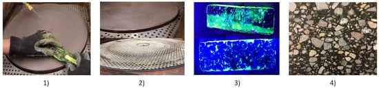
Using specially adapted preparation techniques for asphalt, sections are made from drill cores or laboratory specimens (e.g., Marshall specimens, plates from the rolling sector compactor). The sections should have a width of 100 to 150 mm to provide a representative sample of the structure. A saw with diamond-tipped blades is used to prepare the sections from the test specimens. During the cutting process, water is used as a cooling agent, as the binder in particular, tends to soften during cutting and can thus smear—filling air voids. After cutting, the specimen has to be dried. After drying the air voids are filled by vacuum impregnation with colored and fluorescent epoxy resin. The step is carried out in a vacuum chamber at a minimum pressure of 3 kPa. Any excess epoxy resin is polished off after complete curing (Figure 21), so that the epoxy resin is only present in the filled cavities.
The prepared surface of the polished sections is recorded as a UV scan by a flat board scanner. The generated UV scan is then analyzed with the JMicroVison software (Freeware, Version 1.3.3). The color values are assigned to the pixels; the threshold values set should distinguish between air voids, aggregate, and binder (Figure 32). After adjusting the threshold values, various algorithms are used to extract the individual objects from the entire object. Using digital image processing, all individual cavities are captured and stored in tabular form.
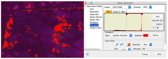
Figure 32.
Identification of air voids using pixel-based segmentation.
This data must then be processed further with other software tools (Matlab (Mathworks, Natick, MA, USA, Version R2021b), Octave (Freeware, Version 6.4.0), Excel (Microsoft, WA, USA, Version 16.55)), which allows, for example, to determine the absolute void content, the vertical, and horizontal void distribution and void orientation [24][3]. The different data types are listed in Table 1.
Table 1.
Data types from the evaluation.
| Type | Details |
|---|
| Area | Expansion of the cut air void area |
| Perimeter | Length of the boundary |
| Length | Longest expansion along the mayor axis |
| Orientation | Angle between the principal axis of an air void and the horizontal |
| Width | Longest expansion along the minor axis |
| Equivalent circular diameter | Diameter of a circle with the same area |
| Feret diameter | Longest expansion along defined orientation |
| Coordinates of the varycenter or centroid | Arithmetic mean position of the air void pixels |
1.2. High-Resolution Computed Tomography (µ-CT)
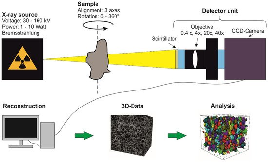
The increasing use of X-ray sources in medicine has also led to the development of high-energy X-ray sources for use in materials science. In order to be able to image the very fine and usually very complex structures with high resolution, so-called X-ray microscopy is often used, in which magnification objectives are used in the detector unit. A scintillation counter is mounted in front of each objective, which converts the X-rays into visible light that is recorded by a CCD camera (charge-coupled divice). Very high magnifications and resolutions can be achieved with this setup (Figure 43).
With µ-CT, single images are generated at different angles by radiating through the sample in different positions. A high radiation absorption of the sample, shows a dark CT signal; with a sample more permeable to radiation, the CT signal becomes brighter. The radiation absorption of a sample depends on various factors such as density, material thickness, and atomic number. The different gray values in a CT image therefore indicate different material densities. The images are acquired with 16 bit and therefore have gray values between 0 and 65535. The magnification of the image section to be viewed can be influenced by varying the projection geometry over the distance between the X-ray source, detector unit, and sample. To perform a 3-D reconstruction, images are taken in an angular range of at least 180°. To minimize artifacts during imaging, samples are usually rotated 360° during measurement. After the measurement, a 3-D image of the sample can be calculated from the individual projections (>1000) using a computer algorithm. The gray values are also inverted in this step, so that areas with a high density appear lighter while low densities are displayed darker.
For the measurements, a high-resolution computer tomograph (µ-CT; see Figure 4 3 for functional principle) type Xradia 520 Versa, Carl Zeiss Microscopy GmbH (Oberkochen, Germany), was used, which has a spatial resolution of ≥0.7 µm. The measuring unit is shown in Figure 54. The X-ray source can be operated with a voltage between 30 and 160 kV at a power of 1 to 10 watts. With a total of 12 filters (6 low-emission and 6 high-emission filters), the X-ray beam can be adapted to the sample properties. A surface detector (magnification factor 0.4×) or three different objectives (4×, 20× and 40×) with scintillators can be used for signal detection. The sample stage can be moved on all three axes so that the region of interest (ROI) of the sample can be targeted. The reconstruction of the acquired projections is then performed automatically or manually with the XMReconstructor software (Zeiss Microscopy GmbH, Oberkochen, Germany, Version 11.1.8043.19515).

For sample preparation, the asphalt samples were sawed into prismatic specimens with a maximum length of 7 cm. The samples of bitumen emulsion with different amounts of tracer were placed between two glass slides. The measurement parameters are summarized in Table 2.
Table 2. Measurement parameters of the µ-CT acquisitions.
| Measurement Parameter | Bitumen Emulsion | Asphalt Sample |
|---|---|---|
| Source setting | 140 kV; 10 watt | 140 kV; 10 wat |
| Source filter | Air | HE 1 |
| Source distance | 50 mm | 125 mm |
| Detector distance | 85 mm | 55 mm |
| Resolution | 25.6 µm | 48.0 µm |
| Optical Magnification | 0.4× | 0.4× |
| Exposure time | 1 s | 6 s |
The data sets are evaluated using the Avizo 9.4 software from Thermo Fisher Scientific Inc. (Waltham, MA, USA). In addition to numerous display options, it offers various filters and segmentation options. By segmenting the individual projections as accurately as possible, models are created, for example of air inclusions in the microstructure or aggregate. These models can then be mathematically evaluated. In addition to various geometric quantities, position parameters and histograms can be generated and custom formulas can be included. In this way, material parameters, such as the aspect ratio of particles, can be output directly without having to calculate them in an additional work step.
For the following investigations, gray value histograms of partial areas of the images were evaluated and compared.
2. Investigation of the Layer Boundaries with Imaging Methods
In road construction, asphalt layers are paved either “hot on cold” or “hot on hot”. In the “hot on cold” paving method, the base is sprayed with bitumen emulsion to bond the two layers together before paving the superstructure. The amount of bitumen emulsion sprayed can vary depending on the type of base.
The aim of the first step of this study was to investigate a suitable method to observe the bonding zone of the asphalt layers and, in particular, to identifying the bitumen emulsion, thus enabling the position of the bitumen emulsion and the contact areas of the bitumen emulsion with the superstructure and the base to be analyzed. For this purpose, initial tactile tests were carried out using the presented imaging methods of asphalt petrology and µ-CT.
2.1. Results of the Investigation of the Layer Boundary by Asphalt Petrology
Using asphalt petrology, initial investigations were carried out on several drill cores. This showed that asphalt petrology is a suitable method for analyzing large asphalt samples. Initial findings on the distribution of air voids can thus be obtained. This allows the compaction of the asphalt layer to be assessed, which has an influence on the layer bond. Furthermore, a rough analysis of the layer boundary is possible. At the layer boundary, the void content, the position and type of voids, and the position of the aggregate can be assessed (see Figure 6 5 red and green arrows), which enable initial conclusions to be drawn about the material behavior at the layer boundary.
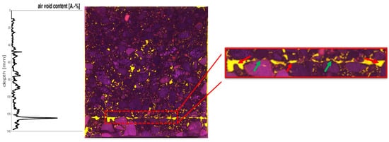
Figure 65.
Analysis of voids over depth using asphalt petrology (red arrows: void analysis; green arrows: location of aggregate).
Asphalt petrology provides a 2-D insight into the sample, which is the basis for assessing the air void structure. The results show that although the asphalt petrology method allows deep insights, they are not sufficient in some cases, especially when identifying very thin (bitumen emulsion) and small components (air voids) in the asphalt structure. For a 3-D observation of a sample, several sections of a sample would have to be generated. This is possible in principle, but components of the sample are lost due to the 2 mm wide saw blade and thus falsify the results.
2.2. Results of the Layer Boundary Analysis by µ-CT
Based on the results of the asphalt petrology studies, further investigations were conducted using a second imaging technique of computer tomography. Since different densities are detected in this method, the layer boundary could only be estimated by an accumulation of pores and aggregate boundaries. Figure 7 6 shows a sectional view of an asphalt sample consisting of a base and a superstructure. The two asphalt layers were bonded to each other via a bitumen emulsion. It can be seen that the aggregate (light gray) is bonded together by the bitumen (dark gray). In the area where the layers are bonded, a higher porosity (black) can be observed. However, the distribution and location of the bitumen emulsion cannot be differentiated.
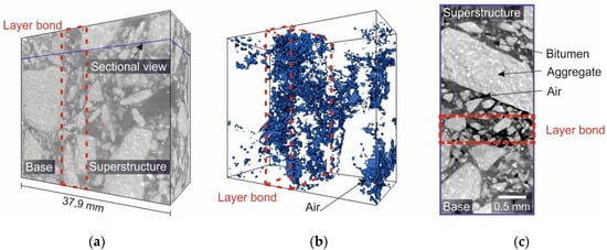
Figure 76. CT-Scan of an asphalt composite sample with a resolution of 42.9 µm: (a) 3-D reconstruction of the sample which provides an overview of the measurement; (b) model of the entrapped air; (c) sectional view into the sample.
3. CT Examinations with Tracer
The results have shown that the consideration of the composite zone in asphalt structures by asphalt petrology does not allow the bitumen emulsion to be identified. The results of the µ-CT showed that due to the identical density of the bitumen emulsion and the bitumen of the asphalt mixture (base; superstructure) of approximately 1.025 g/cm3, it is not possible to clearly observe the bitumen emulsion in particular in the scans. For this reason, in a second step of the study, an option was developed in which the bitumen emulsion in particular becomes visible.
In the scientific field as well as in medicine, the tracer method is well-known, in which a contrast agent of higher density (tracer) is added to the substance to be examined. Due to the difference in density, the area relevant to the investigation becomes visible and can then be analyzed. Castorena, Pape, and Mooney [25][5] added titanium dioxide as a powder to the binder before mixing it into the asphalt concrete in order to investigate the mixing between reclaimed asphalt and fresh asphalt. For this purpose, two mixtures with a high proportion of reclaimed asphalt were investigated using X-ray spectroscopy. Yang and Xu [26][6] also investigated the mixing between reclaimed asphalt and fresh asphalt using infrared analysis of an asphalt mix. The new asphalt was mixed with carboxy-terminated butadiene acrylonitrile (CTBN) as a tracer for identification. Five percent by weight has proven to be suitable.
3.1. Tracer Selection and Specimen Preparation
In the investigations carried out here barium sulphate (BaSO4, barite) was used as a tracer for the bitumen emulsion. The barite was added as a very finely milled powder as well as in the form of coarser barite sand. Both types are characterized by a significantly higher density (4.5 g/cm3) compared to bitumen (1.025 g/cm3) and to aggregate (in the range of 2.5 to 3.0 g/cm3). In addition, barite is chemically inert. The following figure shows the substances pictorially.
The particle size distribution of the barite powder and barite sand (Figure 87) was measured by using a laser granulometer LS 13 320 XR from Beckman Coulter GmbH (Brea, CA, USA) using the wet mode with distilled water. The result was evaluated according to the Mie theory. The differences in particle size distribution can be seen in Figure 98. The barite sand has a significantly coarser particle size distribution compared to the barite powder.
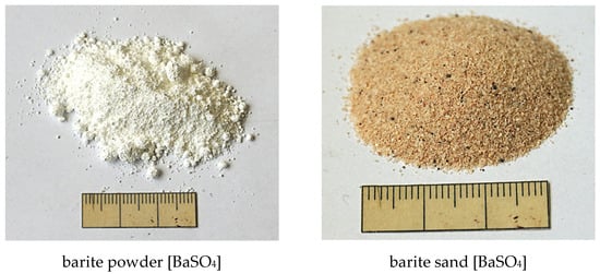
Figure 87.
Tracers with different grain sizes.
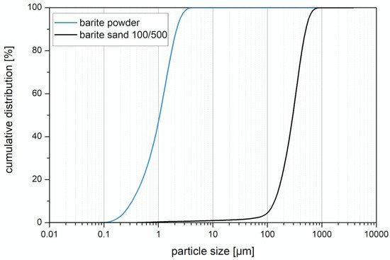
Figure 98.
Particle size distribution of barite powder and barite sand.
To determine the suitability of barite as powder and as sand, the influence on the change of the binder properties was determined on the one hand and the visibility in the µ-CT on the other. For this purpose, the two tracers were added using a high-performance mixer (see Figure 109). The addition of the individual amounts of tracer (see Table 3) was carried out at a speed of 700 rpm. This ensured that the tracer was evenly distributed in the emulsion and that no agglomerates formed.
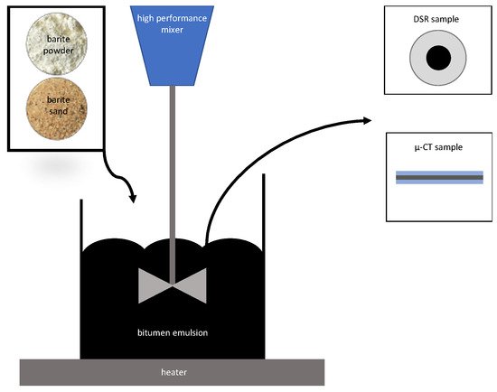
Figure 109.
Schematic drawing of the material preparation.
Table 3.
Addition quantities of the tracers.
| Bitumen Emulsion |
Tracer | Addition Quantity of the Tracer [wt%] |
Addition Quantity of the Bitumen Emulsion [wt%] |
Sample Name |
|---|
| C60 BP4-S | barite powder | 10 | 90 | B10 |
| C60 BP4-S | barite powder | 15 | 85 | B15 |
| C60 BP4-S | barite powder | 20 | 80 | B20 |
| C60 BP4-S | barite sand | 10 | 90 | S10 |
| C60 BP4-S | barite sand | 20 | 80 | S20 |
3.2. Effect of the Addition of Barite Sulfate on Imaging
In order to quantify the influence of barite sulfate on the visibility of bitumen emulsion in CT scans, the samples were measured in the glass panes. For this purpose, the same gray scale definition was used for the minimum and maximum values in the reconstruction of the results. Subsequently, the gray values of the individual samples (Table 3) were analyzed (Figure 11 0 and Figure 112).

Figure 110. Cross-section through the CT scan of the bitumen samples with 10 wt%, 15 wt%, and 20 wt% barite powder (left) and evaluation of the gray scale histograms for the different dosages (right).
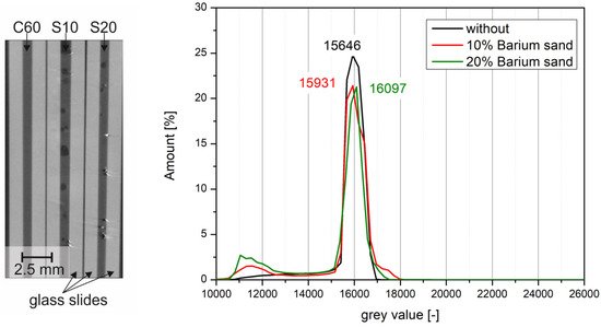
Figure 121. Cross-section through the CT scan of the bitumen samples without and with 10 wt% and 20 wt% barium sulfate sand (left) and evaluation of the gray scale histograms for the different dosages (right).
In the images, the bitumen without tracer (reference) was determined with a peak at a gray value of 15,646. By adding barite powder, the peaks became broader. The addition of 10 wt% barite powder resulted in a slight shift of the gray value to 16,264, but most of it still overlaps with the reference value. After addition of 15 wt%, the peak shifts more clearly into the lighter range and is at 17,490. Here, too, there is still a small overlap area. A complete separation of the peaks was achieved with the addition of 20 wt% barite powder; here the peak was shifted to 19,733.
The addition of barite sand resulted in very small shifts in the peaks from 15,646 (reference) to 15,931 (10 wt%) and 16,097 (20 wt%), respectively. All three peaks are directly above each other so that no distinction could be made between the bitumen emulsions. The air voids that were additionally included in the samples are recognizable (Figure 132). The bitumen emulsion without tracer as well as the one with barium sulfate powder are free of porosity.
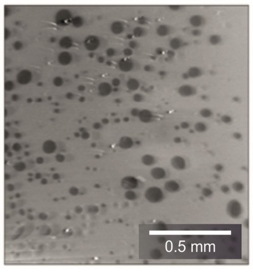
Figure 132.
Sectional view through the bitumen emulsion with 10 wt% coarse barite sand.
3.3. Effect of the Addition of Barium Sulphate on the Binder Properties
In addition to the criterion of imaging with the µ-CT, the influence on the change of the binder properties with the addition of the tracers was investigated. For this purpose, the manufactured test specimens were examined with the dynamic shear rheometer (DSR) in the Temp Sweep according to AL DSR testing (T-Sweep). The test specimens were tested under defined oscillating stress and temperature range. The temperature was increased from 30 to 90 °C. During the test procedure, the complex shear modulus [Pa] and the phase shift angle [°] were determined and subsequently used to evaluate the influence of the addition of the tracer on the binder properties. The phase angle expresses the elastic recovery potential. Ideally elastic materials have a phase angle of 0° and react completely reversibly after the application of load has ended. Purely viscous materials react to the application of force with irreversible deformation. In this case, the phase angle is 90° [27][7]. The results are shown in the Black diagram. The Black diagram offers the advantage of displaying the measured rheological characteristics in one diagram.
The results of the test with the DSR are shown in Figure 14 3 and Figure 154. Figure 14 3 shows the results from the test of adding the barium sulfate as powder. The addition of 10 wt% and 15 wt% does not cause much change in the complex shear modulus and phase angle compared to the results without barium sulfate (red line). The sample with 20 wt% addition shows a lower phase angle to the other samples. This indicates that at addition levels between 15 wt% and 20 wt%, the barite powder has a stiffening effect on the emulsion.
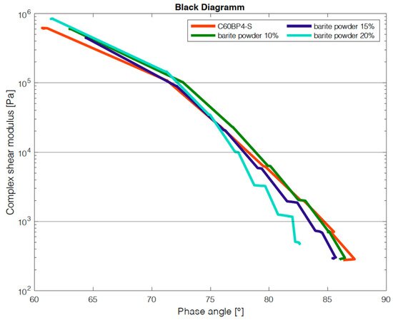
Figure 143.
DSR results of addition of barite powder.

Figure 154.
DSR results of addition of barite sand.
The results of adding barite sand are shown in Figure 154. It is striking that the addition of barite sand does not cause a great change compared to the addition of barite powder. At a small phase angle, the sample with 20 wt% barite sand has a higher shear modulus, but this equalizes again in the course of the test.
References
- Hart, R. Asphaltpetrologie: Einsichten in Asphalt. Straße Autob. 2015, 8, 529–533.
- Tielmann, M.R.D.; Hill, T.J. Air Void Analyses on Asphalt Specimens Using Plane Section Preparation and Image Analysis. J Mater. Civ. Eng. 2018, 30, 04018189.
- Tielmann-Unger, M.R.D. Verbesserte Bestimmung der Hohlraumverteilung von Asphaltprobekörpern. Ph.D. Thesis, Technische Universität Darmstadt, Darmstadt, Germany, 2019.
- Umbach, C.; Middendorf, B. 3D structural analysis of construction materials using high-resolution computed tomography. Mater. Today Proc. 2019, 15, 356–363.
- Castorena, C.; Pape, S.; Mooney, C. Blending Measurements in Mixtures with Reclaimed Asphalt: Use of Scanning Electron Microscopy with X-Ray Analysis. Transp. Res. Rec. J. Transp. Res. Board 2016, 2574, 57–63.
- Yang, Z.; Xu, W. Infrared Spectroscopy Analysis of the Blending of Virgin and RAP Binders in Hot Recycled Asphalt Mixture with CTBN as Tracer. J. Test. Eval. 2019, 47, 20170302.
- Gehrke, M. Komplexe Charakterisierung bitumenhaltiger Bindemittel anhand temperatur-, frequenz- und belastungsabhängiger Kennwerte. Ph.D. Thesis, Ruhr-Universität Bochum, Bochum, Germany, 2017.
More