Your browser does not fully support modern features. Please upgrade for a smoother experience.
Please note this is a comparison between Version 1 by Nam Kim and Version 3 by Rita Xu.
Condition-based maintenance (CBM) is a maintenance policy that maintains the reliability of system operation and reduces the downtime of the system. Prognostics and health management (PHM) has attracted much attention as the enabler of CBM. The PHM aims to predict the remaining useful life (RUL) of the system and suggest an optimal health management strategy.
- system-level prognostics
- performance
- remaining useful life
- dependency
1. Introduction
Condition-based maintenance (CBM) is a maintenance policy that maintains the reliability of system operation and reduces the downtime of the system. Prognostics and health management (PHM) has attracted much attention as the enabler of CBM. The PHM aims to predict the remaining useful life (RUL) of the system and suggest an optimal health management strategy. The PHM consists of four main stages: sensing, diagnostics, prognostics, and health management, which are illustrated in Figure 1. In the sensing stage, PHM engineers determine what to measure and which kind of sensors to install. Health diagnostics is the process of evaluating the degree of damage significance and identifying the root causes of failure. In other words, it focuses on the current operability of the system at stake. On the other hand, health prognostics aims to provide information about the future operability of the system. Prognostics includes establishing a failure precursor which indicates an incipient degradation of the system and estimates the RUL based on the current health state and expected future operating conditions [1]. Finally, the health management of the system is performed based on the information obtained from diagnostics and prognostics. Each step has its own challenges. For example, effective sensor network design for sensing [2], feature extraction, observability analysis, and diagnostics algorithm for fault diagnostics [3][4][5][3,4,5], development of prognostics algorithm [6], and proper system operation strategy for health management [7]. In view of the CBM, however, the prognostics is the most important since it enables the proactive maintenance plan [1][8][1,8]. This article focuses on the prognostics of complex systems that are encountered in the real industry.
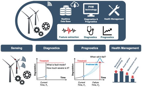
Figure 1. Levels of prognostics and health management.
To date, there are many valuable review papers and books in the PHM with diverse aspects such as the general process of PHM [1][9][10][11][12][13][14][15][1,9,10,11,12,13,14,15], pre-processing [16][17][16,17], and prognostics algorithms [18][19][20][21][22][18,19,20,21,22]. For example, Lee et al. [1] provided a comprehensive review of the PHM followed by an introduction of a systematic PHM design methodology for converting data into prognostic information. Lei et al. [14] provided a systematic review of machinery prognostics from the data acquisition to the RUL prediction and summarized several prognostics datasets commonly used for the research. An et al. [22] presented practical options for prognostics to select an appropriate method for different applications. All the reviews have provided successful case studies and useful descriptions of prognostics algorithms. However, most of the reviews have focused on the component-level prognostics, such as the bearings [23][24][23,24], gears [25][26][25,26], and batteries [27][28][29][27,28,29].
As the industrial systems in the field become more complex, comprising of multiple components, system-level prognostics is gaining much more interest from industry and academia. A complex system is composed of many interlinked components, which makes the system-level prognostics difficult [10][30][10,30]. It should be noted that the degradation and health condition of the system is determined by its components, which means that the individual degradation of components should be explored first and integrated to assess the system performance [10][31][10,31]. From the research viewpoint, the system-level prognostics has different characteristics from those of the component-level as summarized in Figure 2. At the component level, a single or a set of sensors, such as vibration, acoustic emission, and temperature sensors, can be used to monitor damage degradation. Since components are relatively easy to test, a large number of failure data can be obtained from a testbed for the algorithm development. In addition, a dedicated algorithm can be developed for feature extraction of the target component. On the contrary, system-level prognostics contains multiple sensors from various components. Dedicated algorithms may not work in one way or the other in the system. Models are rarely available due to the system complexity, which means that the data-driven method may be the only option. Few or no failure data exist in the real operation or by the testbed. All these are the issues around the system-level prognostics.
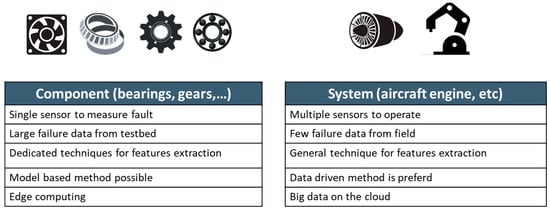
Figure 2. Prognostics approach for component and system level.
2. Approach for System-Level Prognostics
Based on the issues and challenges mentioned in the introduction, this section reviews the approaches that have been addressed to solve the system-level prognostics. It can be grouped into four categories: (1) system health index-based, (2) integration of components’ RUL, (3) prognostics under influenced components, and (4) multiple failure modes. To help readers understand, authors have added simple illustrative examples in each category. It should be noticed that each approach is not about a specific prognostics algorithm but the way to integrate the information from multiple components for system-level information. In this paper, this process is called ‘systematization’. Therefore, any prognostics algorithms can be used before performing the systematization.
2.1. Approach 1: System Health Index-Based Approach
In the system health index-based approach, the health index is introduced to represent the degradation state of the system. Ideally speaking, the system health index should be derived from the degradation of each component. This is however hard to achieve because the relationship between the components and system is usually unknown. Under this circumstance, the system health index-based method can be further divided into three groups: (1) physical system performance (PSP)—physical outputs such as the flow rate of a piping system or the generated power of wind turbine as an example, (2) virtual system performance (VSP)—index representing the system health such as the probability of system failure or distance from the normal; and (3) direct RUL of the system. Among the three groups, the PSP, which employs a physical model, has a strength in both physical interpretation and prediction accuracy. However, such a model is rarely available for complex systems. Thus, the VSP and direct RUL are taken as more practical options, which is also challenging since a large number of run-to-failure data are required.
Figure 3 shows the example of a DC motor to aid in explaining the system health index-based method. It should not be confused that the motor here is regarded as a system consisting of two components: permanent magnet and bearing, whose degradation affects the system performance: the reduction in the output torque of the motor. Typically, the velocity and current are obtained as the CM data. In the PSP method, system health (e.g., the output torque of DC motor, TO
) is estimated via a physical system model, in which the degradation of the components and the resulting system health are evaluated based on the CM data. In the VSP method, virtual system health is commonly introduced between 1 (normal) and 0 (failure) or vice versa, and an empirical model is developed to relate the CM data with the system health using the run-to-failure data set. For this, a machine learning algorithm whose inputs are features extracted from signals and output is health index between 0 and 1 is usually employed.
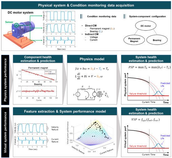
Figure 3. System health index-based approach.
While the overall summaries for each approach in the literature are given in Table 1, a few papers are explained in more detail. In the PSP approach, Rodrigues [32][64] estimated system RUL using the system-level performance indicator obtained by the system model. He converted the health factors of individual components into the performance indices and combined them into the system-level performance. Khorasgani et al. [31] developed a two-step process for the system prognosis. In the estimation step, the system state and degradation parameters are estimated based on the system model using the PF. Then in the prediction step, the first-order reliability method (FORM) is applied to predict the system RUL. In their work, the system EOL was defined based on the system performance, which was calculated from the individual components and system degradation model. Wang et al. [33][65] introduced a Bayesian network-based lifetime prediction method for systems, which combines multiple sensor information and considers the interdependency between accidental failure and degradation failure mechanism. Liu et al. [34][66] developed a dynamic reliability assessment approach for the multi-state system by utilizing the system-level observation history. The proposed recursive method dynamically updates the reliability function of the system by incorporating system-level inspection data.
Table 1. Summary of system health index-based approach.
| Approach | System in the Study | Data Sources | Prognostics Algorithm | |
|---|---|---|---|---|
| Physical System Performance | Water piping system | Direct CM | Dynamic reliability assessment [34] | Dynamic reliability assessment [66] |
| Pump system | Direct CM | Gamma process [32] Similarity-based method [35] | Gamma process [64] Similarity-based method [78] |
|
| Rectifier system | Direct CM | First-order reliability method (FORM) [31] | ||
| Air conditioning system | Direct CM | Gamma process [32] | Gamma process [64] | |
| Virtual System Performance | Punching system | Direct CM | Bayesian network [36] | Bayesian network [79] |
| Unmanned aerial vehicle system | Direct/Indirect CM data & environmental data |
Bayesian network [33] | Bayesian network [65] | |
| Compressor system | Indirect CM data | Similarity-based method [37] | Similarity-based method [80] | |
| Train door system | Indirect CM data | Generative adversarial network [38] | Generative adversarial network [81] | |
| Elevator door motion system | Indirect CM data | Autoregressive-moving average model [39] | Autoregressive-moving average model [67] | |
| Aircraft engine (CMAPSS) | Indirect CM data | Similarity-based method [40][41][42] Particle filter [43][44] General path model [45] Ensemble of data-driven algorithm [46][47] Generative adversarial network [48] | Similarity-based method [47,58,68] Particle filter [52,82] General path model [71] Ensemble of data-driven algorithm [77,83] Generative adversarial network [84] |
|
| Direct Remaining Useful Life | Aircraft engine (CMAPSS) | Indirect CM data | Multi-layer perceptron (MLP) [49][50] Recurrent neural network (RNN) [51][52] Long short-term memory (LSTM) [53][54][55] Convolutional neural network (CNN) [56][57] | Multi-layer perceptron (MLP) [72,73] Recurrent neural network (RNN) [40,76] Long short-term memory (LSTM) [42,46,56] Convolutional neural network (CNN) [74,75] |
In the VSP approach, a virtual system health index is mainly introduced that varies between 1 in the early period and 0 near the failure. Then, logistics regression [39][67] or linear regression [42][68] are used as an empirical system model to convert the CM data into 1D system performance. The elevator door [39][67] or aircraft engine [42][68] are chosen for the demonstration. Other researchers have employed the concept of distance from the normal as the health indicator, which is determined by multivariable state estimation technique (MSET) [58][69], auto-associative kernel regression (AAKR), or auto-associative neural networks (AANN) [59][45][70,71]. The direct RUL method is similar to the VSP but the RUL is employed directly instead of the VSP. That is, the CM data are directly related with the RUL of target assets using artificial intelligence (AI) algorithms, such as multi-layer perceptron (MLP) [49][50][72,73], convolutional neural network (CNN) [56][57][74,75], recurrent neural network (RNN) [51][52][40,76], and long short-term memory (LSTM) [53][54][55][42,46,56], in which the system-model is considered as a black-box. There have also been studies in which the health index is first developed for the system, and the RUL prediction by the index is followed using such as the particle filter [43][52], the similarity-based method [40][41][42][47,58,68], and the ensemble approach [46][77]. It should be remarked that although these papers address the system in their study, it is not strictly the system prognosis since they treat the system as a single unit without considering the components.
2.2. Approach 2: Integration of Components’ RUL into the System
The second approach is to integrate RUL information of individual components to obtain the system-level RUL, rather than directly determining the system health index or RUL as in approach 1. Figure 4 briefly illustrates the component RUL-based approach. In the figure, two examples of the serial and parallel system are given, which define the system failure based on the ‘AND’ and ‘OR’ gates of the fault tree diagram. For the gearbox system in Figure 4a, failure of any components results in system failure. In this case, the union of three RULs yields the system RUL. For the aircraft hydraulic system with redundancy, the failure of all three sub-systems leads to system failure as shown in Figure 4b, which means that the intersection of three RULs gives the system RUL.
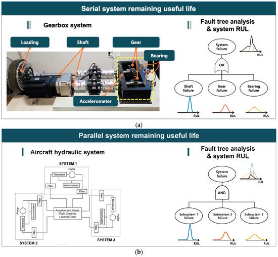
Figure 4. Component RUL-based approach: (a) System RUL of serial systems (gearbox system); (b) System RUL of parallel systems (aircraft hydraulic system).
The diagram can be generalized to the complex system by applying the fault tree analysis (FTA), in which the component-level RULs are propagated to the system RUL by the fault tree structure (see, e.g., Gomes et al. [60][85]). Ferri et al. [61][86] proposed a methodology for maintenance planning in the view of system-level prognostics using the FTA. In the end, the system-level RUL was used to identify optimum component combinations to be repaired in order to maximize system safety. In this category, some literature has employed a physical system model to determine the RUL of individual components. This approach, however, results in a higher computational burden as the number of components increases. To overcome this issue, model decomposition methods have been proposed by Daigle et al. [62][63][64][87,88,89], in which a distributed approach is developed for the system-level prognostics by decomposing both the estimation and prediction problems into computationally independent sub-scale problems. Then the system RUL is determined as a minimum of the independent subsystem’s RUL. They have also developed PF-based prognostics characterizing multiple damage progression paths based on the joint state-parameter estimation [65][90]. Vasan et al. [66][91] proposed approaches based on decomposing the system into multiple critical circuits and exploiting the parameters specific to the system’s circuits. Chiachio et al. [67][92] introduced a mathematical framework for modeling prognostics at a system level based on the plausible Petri net by incorporating maintenance actions, various prognostics information, expert knowledge and resource availability. Table 2 summarizes the component RUL-based methods for system-level prognostics.
Table 2. Summary of component RUL-based approach.
| System in the Study | Algorithm | Characteristics | |
|---|---|---|---|
| Aircraft ECS | Fault tree analysis & Kalman filter [60] | Fault tree analysis & Kalman filter [85] |
Fault tree-based RUL fusion Independent failure event |
| Aircraft hydraulic system | Fault tree analysis & Kalman filter [68] | Fault tree analysis & Kalman filter [93] | Individual component’s RULs are estimated using Kalman filter and system-level RUL is determined based on Fault tree analysis |
| Electrical power system | Fault tree analysis [61][69] | Fault tree analysis [86,94] | Fault tree-based RUL fusion Optimum component combination to repair |
| Kalman filter [70] | Kalman filter [95] | Individual component’s RUL is estimated using Kalman filter and defined as system-level RUL | |
| Four-wheeled rover | Model decomposition [62] | Model decomposition [87] | Decomposition of a large prognostics problem into several Independent local subproblems |
| Pump | Model decomposition [63] | Model decomposition [88] | Novel distributed model-based prognostics scheme The system RUL is the minimum of all the distributed subsystem RULs |
| National Aerospace System | Model decomposition [64] | Model decomposition [89] | Combining individually independent components RULs of aircraft environmental control system |
| Centrifugal pump | Particle filter [65] | Particle filter [90] | Individual component’s RULs are represented as particles and system-level RUL are approximated by them. |
| RF receiver system | Model decomposition [66] | Model decomposition [91] | Decomposing a system-level problem into multiple critical components |
| Numerical example | Petri net [67] | Petri net [92] | Incorporation of maintenance actions, various prognostics information, expert knowledge and resource availability |
2.3. Approach 3: Prognostics under Influenced Components
As mentioned before, system-level prognostics is difficult due to the inter-dependencies between the “affecting” and “influenced” components in the system [10][31][10,31]. Such dependencies may lead to the different degradation of the system than the case otherwise. Figure 5 shows the gearbox system, which consists of gear and bearing, where the degradation or fault of bearing affects the degradation of gear. In the figure, if the bearing stays in the normal condition, the health trend of gear shows the normal degradation pattern. When a fault occurs in the bearing, however, the degradation pattern of gear is changed, i.e., is accelerated, and reaches the threshold earlier. This issue has already been studied extensively in the field of maintenance strategies and policies with the topic of the multiple components [71][96]. However, they did not consider the interdependency of the components in the prognostics or RUL prediction.
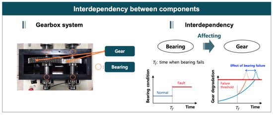
Figure 5. Influenced component-based approach.
While the list of papers for this approach is given in Table 3, some of them are explained in detail as follows. Tamssaouet et al. [72][73][74][75][76][77][97,98,99,100,101,102] proposed a methodology based on the inoperability input-output model to evaluate the system-level RUL in the situation where multiple interactions between components and the influence of the environment exist. Liu et al. [78][103] introduced dynamic reliability assessment and RUL prediction of a system that consists of a pump and valve. Parallel Monte Carlo simulation and recursive Bayesian method are integrated for the purpose of failure prognostics under dependency among components. Hu et al. [79][104] proposed a failure prognosis method using the dynamic Bayesian network (DBN) for a complex system, which considers the interaction between components and influence of protection action in the system during dynamic failure scenarios. Maitre et al. [80][105] emphasized that when one component has a failure, the remaining components compensate for the loss of the component and thus function in a ‘boosted’ mode. As a result, the component under ‘boosted’ mode shows a more severe degradation than without it. Hafsa et al. [81][106] emphasized the importance of interactions between components in RUL prediction. They proposed a method combining the probabilistic Weibull and stochastic dependency model, which characterizes the effects of degradation interaction derived from other components. Hanwen et al. [82][107] demonstrated that there exists a noise that impacts the system with multiple components, as all the components operate in the same circumstance and affect each other. They named this public noise. To describe the degradation with public noise, Brownian motion that affects the degradation of components was added to the Wiener process. Then, the degradations of the components are jointly estimated by the KF, and the system RUL is determined by the minimum RUL of components. Bian and Gebraeel [83][84][108,109] proposed a stochastic modeling methodology considering interactions among the degradation of components in a system. They focused on characterizing the relationship between the influencing and the affected component.
Table 3. Summary of prognostics of influenced components approach.
| System in the Study | Algorithm | Characteristics | |
|---|---|---|---|
| Tennessee Eastman Process | Inoperability input-output model [72][73][74][75][76][77] | Inoperability input-output model [97,98,99,100,101,102] | Interaction between components Influence of the environment |
| Pump & Valve | Parallel Monte Carlo simulation &dynamic reliability assessment [78][85][86] | Parallel Monte Carlo simulation &dynamic reliability assessment [103,110,111] | Interaction between components |
| Flue gas energy recovery system | Bayesian network [79] | Bayesian network [104] | Interaction between components Influence of the protection |
| Lorry system | Webuill model & Stochastic dependency model [81] | Webuill model & Stochastic dependency model [106] | Interaction between components |
| Blast furnace wall | Multi-degradation modeling with public noise [82] | Multi-degradation modeling with public noise [107] | Interaction between components |
| Hydraulic hybrid system | Bond graph [87] | Bond graph [112] | Interaction between components Dependency on operating mode |
| Gearbox | Marshall-Olkin bivariate exponential distribution [88] | Marshall-Olkin bivariate exponential distribution [113] | Interaction between failure mode |
| Aircraft bleed system | System redundancy & Adaptation of operational modes in degraded functioning [80] | System redundancy & Adaptation of operational modes in degraded functioning [105] | Interaction between components |
| Cold box unit in petrochemical plant | Regression [89] | Regression [114] | Interaction between components |
| Numerical simulation | Structural impact measure [90] Stochastic modeling of interaction [83][84] | Structural impact measure [115] Stochastic modeling of interaction [108,109] |
Interaction between components |
2.4. Approach 4: Prognostics of Multiple Failure Modes
In the PHM, identification of fault modes is the initial step toward successful prognostics [41][58]. In many cases, the system contains multiple failure modes even for a single component. In that case, the degradation of components or systems can show a different pattern from those of single mode, which should involve identifying active failure modes and tracking their progression. The case is illustrated by an example in Figure 6, where the bearing faults can occur at different places with different progression paths such as the outer race, inner race, and rolling element. The faults if occurred concurrently can interact and accelerate the global degradation of the components [65][90].
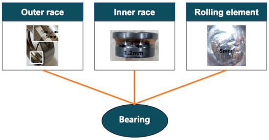
Figure 6. Illustration of failure mode-based approach.
For accurate fault prognosis, the method should be able to address this aspect. Several approaches have been studied to this end, most of which were however rooted in the traditional reliability engineering such as a hazard model or survival analysis [91][92][93][94][116,117,118,119]. Ragab et al. [91][116] merged the logical analysis of data with a set of non-parametric cause-specific survival functions and applied it to the bearing prognostics whose failure modes were inner race, outer race, and rolling element faults. Zhang et al. [93][118] presented a mixture Weibull proportional hazard model for the EOL estimation of mechanical system that includes multiple failure modes and applied to a pump system that contains two failure modes: sealing ring wear and thrust bearing damage. Historical lifetime and condition monitoring data were combined into the traditional proportional hazard model. Blancke et al. [95][120] introduced a multi-failure mode prognosis approach for complex equipment. They used graph theory and stochastic models for diagnostics and prognostics, respectively. Once the failure mechanism is detected by the diagnostic process, the prognostic algorithm based on a stochastic model is used to predict the possible failure mode dynamically as new data are acquired. The proposed algorithm was applied to a hydroelectric generator stator, which contains more than 150 failure mechanisms associated with three failure modes. While the above studies are based on the traditional reliability approach, there have been other studies for the multiple failure modes prognosis by using the PF [65][96][97][98][90,121,122,123]. Daigle and Goebel [98][123] used the PF for model-based prognostics of a valve system that contains multiple failure modes. Zhang et al. [96][121] introduced PF-based multi-fault prognostics of bearing degradation whose failure modes were grease damage, spall, and unknown fault. They monitored features directly related to each failure mode and utilized them in the PF framework. Table 4 summarizes the system-level prognostics considering multiple failure modes.
Table 4. Summary of failure mode-based approach.
| System in the Study | Algorithm | Types of Failure Mode | |||||
|---|---|---|---|---|---|---|---|
| Rolling element bearing | Survival analysis [91] | Survival analysis [116] | Inner race fault Outer race fault Rolling element fault |
||||
| Particle filter [96] | Particle filter [121] | Grease breakdown Spall Unknown fault |
|||||
| Pump system | Proportional hazard model [93] | Proportional hazard model [118] | Sealing ring wear Trust bearing damage |
||||
| Electronic Throttle Control | Proportional hazard model [92][94] | Proportional hazard model [117,119] | Accelerator pedal Throttle Body Other three failure |
||||
| Valve system | Particle filter [98] | Particle filter [123] | Spring rate Internal leak Top (bottom) external leak Friction |
||||
| Ion mill etching system (PHM Data challenge 2018) | Recurrent neural network (RNN) [99][100] Long short-term memory (LSTM) | 125 | [101] Convolutional neural network (CNN) [ | ] Long short-term memory (LSTM) [126 | 102] | Recurrent neural network (RNN) [124,] Convolutional neural network (CNN) [127] |
Flow pressure drop Flow pressure high Flow leakage |