Your browser does not fully support modern features. Please upgrade for a smoother experience.
Please note this is a comparison between Version 2 by Bruce Ren and Version 1 by Sulaiman Matarneh.
Preservation of meat through freezing entails the use of low temperatures to extend a product’s shelf-life, mainly by reducing the rate of microbial spoilage and deterioration reactions. Characteristics of meat that are important to be preserve include tenderness, water holding capacity, color, and flavor. In general, freezing improves meat tenderness, but negatively impacts other quality attributes. The extent to which these attributes are affected depends on the ice crystalline size and distribution, which itself is governed by freezing rate and storage temperature and duration.
- preservation
- crystallization
- freezing/thawing
- meat quality
- freezing technologies
1. Introduction
Preserving food to extend its shelf-life has been practiced for several millennia. At its roots, food preservation involves altering the product’s inherent properties, mainly pH and water activity (Aw), in order to inhibit the growth of pathogenic microorganisms, molds, and spores. Preservation techniques are also used to control chemical reactions involved in deteriorating food products, such as lipolysis, lipid oxidation, and proteolysis [1]. An example where both intrinsic hurdles (pH and Aw) are modified is during the processing of semidry and dry fermented meat products, in which the product is typically inoculated with a microbial culture to lower the pH, and subsequently dried (lowering Aw) [2]. However, alteration of the product’s inherent properties to this extent means that it is no longer viewed as “fresh”, a term generally preferred by consumers to be associated with their food [3], particularly concerning meat products. Alternatively, food products can be preserved without the need of making significant changes to their inherent properties when stored at very low temperatures. Although preservation through freezing is applicable to a variety of food commodities, this review focuses on the freezing of fresh meat.
Due to the large amount of water in fresh meat, ~60−70% on a wet basis [4], meat products are prone to microbial spoilage and chemical reactions that can negatively affect aspects of meat quality, such as its color, texture, and flavor [5]. Freezing is extensively utilized by the meat industry as a method of preservation during transport and storage. Nonetheless, freezing can adversely affect the very same quality characteristics that it was meant to preserve, resulting in products that are dissatisfying to consumers [6]. Thus, extensive time and research have been dedicated to understanding the physical and biochemical changes occurring in meat during the freezing process and the etiology of these changes [7].
2. Freezing and Crystallization Behavior of Water
By definition, the process of freezing refers to the decrease in molecular motion of existing molecules within an environment [8]. In muscle food, this mainly refers to the decrease in random motion of water molecules that exist within the tissue. The freezing of water in meat can be summarized into three distinct chronological stages: (1) the cooling of the product to its freezing point, (2) the phase transition stage in which latent heat is removed, and (3) the product reaching the final temperature of storage (tempering) [9]. It is during the transition stage that water molecules are oriented in a crystalline manner, and ice crystals are formed. Within the crystallization stage, the phenomenon of nucleation and crystal growth occurs. In the context of water freezing, nucleation refers to the formation of an “embryo”, or nucleus ice crystal, that can later grow into a larger ice crystal [10]. There are two forms of nucleation that can occur, namely primary and secondary nucleation. Primary nucleation refers to the formation of new crystals within the medium in which no preexisting crystals are present. Once a crystalline structure has been formed, a sudden breakage of the structure can catalyze the formation of new crystals. This phenomenon is referred to as secondary nucleation, and requires less energy to form stable nuclei relative to primary nucleation [10]. Similarly, in a complex matrix with various constituents (e.g., proteins and minerals), similar to that of a food system, these constituents can also lower the energy required to form a nucleus, and assist with secondary nucleation [11]. In both cases, supercooling, which is defined as the subtle decrease in temperature as a result of the initial arrangement of water crystals, is the driving force necessary for nucleation [12]. The rate of nucleation (β) for both primary and secondary nucleation can be modeled using Equation (1), where ΔGc is critical free energy for nucleation, k is the Boltzman constant (1.380649 × 10⁻²³ J/K), T is temperature, z is the Zeldovich factor (which is defined by the relationship between the number of nuclei in both equilibrium and steady-state distribution with respect to surface tension temperature, concentration, Avogadro number, and surface area), f* is the frequency of monomer attached to a nucleus, and C0 is the number of nucleation sites [9]. In summary, Equation (1) implies that the rate of nucleation is a statistical phenomenon, with a higher probability for nucleation to occurring in a system with greater supercooling. (1)
Once formed, the nuclei provide a foundation for which further crystallization can occur, thereby allowing the crystals to grow [13]. Nucleation and crystal growth are two inversely related phenomena that are driven by the rate of supercooling, with more nucleation occurring at greater supercooling rates the smaller the crystal sizes. Therefore, the rate of supercooling is a key factor to consider when determining crystal growth, as it can dictate ice crystal size, distribution, and morphology [9]. Equation (2) is a theoretical model that incorporates supercooling as one of the main determinants of crystalline growth, where G is defined as the rate of crystal growth (°C/min), ΔTs is the supercooling temperature (freezing point temperature [Tf]—nucleation temperature [Tn]), and β (growth constant) and n (growth order) are constants that are experimentally determined [9]. For a more in-depth explanation of nucleation and growth of water crystals, refer to a review by Kiani and Sun [9], which thoroughly describes modeling approaches for nucleation and crystal growth.
(1)
Once formed, the nuclei provide a foundation for which further crystallization can occur, thereby allowing the crystals to grow [13]. Nucleation and crystal growth are two inversely related phenomena that are driven by the rate of supercooling, with more nucleation occurring at greater supercooling rates the smaller the crystal sizes. Therefore, the rate of supercooling is a key factor to consider when determining crystal growth, as it can dictate ice crystal size, distribution, and morphology [9]. Equation (2) is a theoretical model that incorporates supercooling as one of the main determinants of crystalline growth, where G is defined as the rate of crystal growth (°C/min), ΔTs is the supercooling temperature (freezing point temperature [Tf]—nucleation temperature [Tn]), and β (growth constant) and n (growth order) are constants that are experimentally determined [9]. For a more in-depth explanation of nucleation and growth of water crystals, refer to a review by Kiani and Sun [9], which thoroughly describes modeling approaches for nucleation and crystal growth.
 (2)
(2)
3. Energy Balance and Heat Transfer during Water Crystallization in Meat
In general, the thermal center of a product is a point of reference for determining when the completion of freezing occurs, and thus establishing the optimal freezing time [14]. The alternative to this would be to take a series of temperature measurements across the entire object, and establishing an average mass temperature. However, the average mass temperature has the disadvantage of requiring extensive data collection in order to provide precise and accurate estimations [14,15][14][15]. Therefore, thermal center measurements are used more often when establishing freezing time [16]. The total time required for a product to reach the set freezing temperature at the thermal center is known as the effective/standard freezing time [17]. Meat products vary in size and shape, and subsequently the rate of freezing also varies considerably between products. Thus, an effort has been made to establish better freezing practices in order to achieve high-quality products. In this regard, modeling approaches have been created to predict the freezing time for various products. Primarily, heat and mass transfer modeling have been used [18,19,20][18][19][20].3.1. Energy Balance
Equation (3) can be used to calculate the amount of heat to be removed from any food sample: (3)
(3)
where Q is the heat to be removed (kJ), ms is the mass of solids in the sample (kg), cp,s and cp,w are the values of specific heat of the solids and water (kJ/(kg·°C)), respectively, λw is the enthalpy of crystallization or fusion of water at the crystallization temperature (kJ/kg), Ti is the initial temperature of the sample above the crystallization temperature (°C), Tc is the water crystallization temperature (°C), and Tf is the final temperature of the sample below the water crystallization temperature (°C). It is important to emphasize that the values of specific heat may not be constant in a given range of temperatures, and the specific heat of a substance can change with a change in phase [21,22][21][22].
As can be expected, the presence of solutes in food samples can substantially alter the crystallization temperature of the water they contain, causing it to have a lower value than the crystallization temperature of pure water. In general, the deviation of the crystallization temperature from that of pure water depends on the type of solutes present (their molecular weight) and their concentration [23]. Likewise, the values of specific heat of the solids depend on their specific components and their physical state. Several equations have been reported to predict crystallization temperatures of water in foods, and for calculating specific heat values below and above the corresponding crystallization temperature [24,25][24][25].
Even though it is possible to predict the thermal properties of foods (such as water crystallization temperature and specific heat) with empirical equations as explained earlier, the realistic amount of total removable heat required to freeze a sample may deviate from the calculated Q value of Equation (3) (which can be seen as a theoretical value or a simplification). Figure 1 shows the freezing curves of pure water and a food sample. As heat is removed from the food sample, water starts to crystallize at an initial crystallization temperature. At a certain point, the crystallization temperature begins to decrease due to having a more concentrated solution, and crystallization will come to a stop unless more heat is removed from the system. If more heat is removed, one or more eutectic temperatures (the temperature at which there is a coexistence of liquid and solid phases) may be reached. After the eutectic temperatures have been reached, all of the components exist in solid form, and the temperature may continue to decrease as more heat is removed after all the components have undergone crystallization [21].
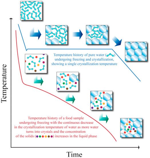
Figure 1. Temperature history of pure water and a food sample during freezing. Adapted from Heldman and Singh [21].
3.2. Heat Transfer and Water Crystallization in Meat
The rate of heat transfer or freezing rate is influenced by the temperature gradient between the product and the freezing medium, the modes of heat transfer involved (convection, conduction, radiation, or their combination), the shape and size of the product as well as its packaging material, and the thermal properties of the product. The fact that many thermal properties (e.g., specific heat, thermal conductivity, and enthalpies of phase change) vary with changes in temperature can make the determination of rates of heat transfer challenging. This, in turn, has created the need to develop simplified solutions to calculate rates of heat transfer and times required to freeze a product. These solutions usually assume the thermal properties to be constant as a function of temperature [21].
The governing equations of heat transfer due to conduction for regular geometries are shown below. Equation (4) corresponds to Cartesian coordinates (rectangular geometries), Equation (5) corresponds to cylindrical coordinates, and Equation (6) applies to a spherical system [26].
 (4)
(4)
 (5)
(5)
 (6)
(6)
(4)(5)(6)Equations (4)–(6) relate the rate of heat transfer in the three dimensions of the corresponding coordinate systems and the heat generated within g˙
(W/m3), with the change in heat content in the corresponding working volume (right side of the equations). If a change in phase (such as water crystallization during freezing) takes place, that would need to be incorporated in the right side of the equations as the total change in enthalpy. To overcome the lack of accuracy from the use of empirical models to predict thermal properties and calculate indirect changes in heat content, thermal analysis seems to be the best approach to determine the exact amount of heat to be removed to reach a defined level of water crystallization. Some of the most frequently used thermal analysis techniques include Differential Scanning Calorimetry (DSC), Differential Thermal Analysis (DTA), and Thermogravimetric Analysis (TG) [27]. Once the total change in enthalpy from a freezing process is determined through any of these thermal analysis techniques, it can be simply taken into account for freezing time calculations. Thermal analyses allow an accurate determination of energy supply or removal requirements [27,28][27][28]. Hobani and Elansari [29] examined the enthalpy change from –40 to 40 °C of meat through Modulated Differential Scanning Calorimetry (MDSC). These authors were able to determine the heat content (which accounted for the freezing and crystallization of water) as a function of moisture, and accurately predicted the changes in specific heat along the temperature range studied.
By analytically solving the governing equations above, it is possible to determine the rates of heat transfer and temperature distributions in an object, and if it is established that heat transfer only takes place in one dimension (which in many situations can be a safe assumption), those analytical solutions can be more easily determined. The analytical solutions of the governing equations involve performing the corresponding energy balance in the working volume, applying the known boundary conditions, and solving the differential equation to determine the corresponding integration constants. The analytical solutions are also known as exact solutions since they agree with the boundary conditions of the differential equations [30]. An example of a widely used analytical solution for regular geometries is Plank’s Equation (Equation (7)), which can be used to calculate freezing times assuming that heat transfer is unidimensional [21,23][21][23]:
 (7)
where tF is the freezing time, ρ is the object’s density, TF is the initial freezing point, T∞ is the cooling medium temperature, a is the characteristic length of the object (the thickness for the case of a slab, or the diameter in the case of a cylinder or a sphere), P and R are constants that depend on the object’s geometry (slab, cylinder or sphere), h is the convection heat transfer coefficient of the cooling medium (which may need to be determined experimentally), and k is the object’s thermal conductivity.
Other analytical, semi-analytical, and empirical methods for freezing time calculation include a modification of Plank’s equation by Cleland and Earle, the method of Lacroix and Castaigne, the method of Pham, the method of Salvadori and Mascheroni, the method of Hung and Thompson, the method of Ilicali and Saglam, the Neumann method, the Tao solutions, the Tien solutions, and the Mott procedure [21,31][21][31]. These methods can be applied to objects with regular shapes (slabs, cylinders, or spheres). Other methods have been developed that can be applied to predict freezing times of objects with irregular shapes, and include the methods of Cleland and Earle, Cleland et al., Hossain et al., and Lin et al. [31].
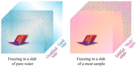
The main advantage of most analytical, semi-analytical, and empirical solutions is their simplicity, but they also have limited applicability in real situations. Many of them require the system or object being studied to have a regular geometry, which may be very unlikely for biological systems. Additionally, many analytical solutions (such as Plank’s equation) assume the physical and thermal properties (such as density, crystallization temperature, thermal conductivity, specific heat, and enthalpies of crystallization) to be constant, which may be an oversimplification that can cause substantial deviations from real measurements, and may not take into consideration the changes in enthalpy due to sensible heat above and below the crystallization temperature. Moreover, analytical solutions assume steady-state heat transfer, a condition that implies that the temperature distribution throughout the system remains constant over time, which is another ideal scenario rarely found in real situations [21,30][21][30]. Additionally, for the specific case of meat and other biomaterials (cellular tissues), the complexity of their structure generates an even greater deviation from the results obtained in analytical solutions, which also assume samples or objects with a homogeneous mass. This feature could only be expected in a pure substance. In reality, meat samples may exhibit micro-regions or “mushy” regions where crystallization and/or solidification may take place in separated areas, rather than uniformly [26], as shown in Figure 2.
(7)
where tF is the freezing time, ρ is the object’s density, TF is the initial freezing point, T∞ is the cooling medium temperature, a is the characteristic length of the object (the thickness for the case of a slab, or the diameter in the case of a cylinder or a sphere), P and R are constants that depend on the object’s geometry (slab, cylinder or sphere), h is the convection heat transfer coefficient of the cooling medium (which may need to be determined experimentally), and k is the object’s thermal conductivity.
Other analytical, semi-analytical, and empirical methods for freezing time calculation include a modification of Plank’s equation by Cleland and Earle, the method of Lacroix and Castaigne, the method of Pham, the method of Salvadori and Mascheroni, the method of Hung and Thompson, the method of Ilicali and Saglam, the Neumann method, the Tao solutions, the Tien solutions, and the Mott procedure [21,31][21][31]. These methods can be applied to objects with regular shapes (slabs, cylinders, or spheres). Other methods have been developed that can be applied to predict freezing times of objects with irregular shapes, and include the methods of Cleland and Earle, Cleland et al., Hossain et al., and Lin et al. [31].
The main advantage of most analytical, semi-analytical, and empirical solutions is their simplicity, but they also have limited applicability in real situations. Many of them require the system or object being studied to have a regular geometry, which may be very unlikely for biological systems. Additionally, many analytical solutions (such as Plank’s equation) assume the physical and thermal properties (such as density, crystallization temperature, thermal conductivity, specific heat, and enthalpies of crystallization) to be constant, which may be an oversimplification that can cause substantial deviations from real measurements, and may not take into consideration the changes in enthalpy due to sensible heat above and below the crystallization temperature. Moreover, analytical solutions assume steady-state heat transfer, a condition that implies that the temperature distribution throughout the system remains constant over time, which is another ideal scenario rarely found in real situations [21,30][21][30]. Additionally, for the specific case of meat and other biomaterials (cellular tissues), the complexity of their structure generates an even greater deviation from the results obtained in analytical solutions, which also assume samples or objects with a homogeneous mass. This feature could only be expected in a pure substance. In reality, meat samples may exhibit micro-regions or “mushy” regions where crystallization and/or solidification may take place in separated areas, rather than uniformly [26], as shown in Figure 2.
 To overcome the limited accuracy and applicability of analytical solutions, numerical methods can be employed, which involve the division of the studied object or medium into small subdivisions that result in the same number of algebraic equations for the unknown temperatures at the nodes located in the interfaces of such subdivisions. These equations can then be solved through computational methods to determine the temperature distributions within the medium. Some frequently employed numerical methods are the finite difference method, the finite element method, the boundary element method, the finite volume method, and the energy balance method [30,32][30][32]. These methods can be applied under steady or unsteady state conditions, thereby allowing for the computation of freezing times. The majority of the currently available computational tools and software use the finite element method and the finite volume method [32,33][32][33]. Application of numerical methods also requires the knowledge of the initial and boundary conditions of the process or phenomenon being studied. Some commonly used initial and boundary conditions include the initial or specified temperature boundary condition, the heat flux boundary condition, the convection boundary condition, the radiation boundary condition, the combined radiation and convection boundary condition, the combined heat flux, radiation and convection boundary condition, and the interface boundary condition [30].
The numerical solutions of the partial differential equations (such as Equations (4)–(6)) that describe physical phenomena can be used to perform virtual or computational simulations of a variety of processing operations, including freezing. Knowing the necessary energy to be removed from a food sample to reach a specific temperature (and/or the physical and thermal properties of the studied food item), as well as the environmental conditions (such as convective heat transfer coefficients and freezing medium temperature), it is possible to predict the time-temperature histories. These predicted values can then be validated in a real experiment, which represents substantial savings in time, material, and labor resources [32].
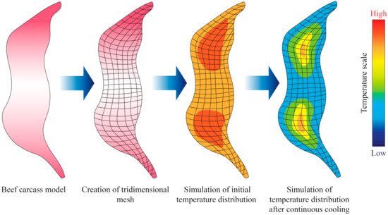
Sun and Zhu [34] conducted computational simulations to determine the freezing time of beef samples with different muscle fiber orientations (parallel to the heat transfer direction and perpendicular). In their study, heat transfer was assumed to be unidirectional in Cartesian coordinates (Equation (4)), and applied the finite difference method with a Crank–Nicholson formulation. They also took into consideration changes of thermal conductivity with temperature. Overall, their results showed a good fit with the predicted simulation that was utilized. However, other studies took into consideration mass transfer phenomena in their modelling approach, as water may either condensate or evaporate from the surface of meat samples during freezing or thawing. Delgado and Sun [35] applied the explicit finite difference method to perform simulations of simultaneous heat and mass transfer during thawing of mild cured ham samples, and the experimental data exhibited a good fit with the partial differential equation applied. More recently, Trujillo and Pham [36] conducted an evaluation of the chilling process of a beef carcass through Computational Fluid Dynamics (CFD), which involved simultaneous heat and mass transfer. The tridimensional geometry of the beef carcass was built in the software the authors employed through established correlations between the different parts of the carcass (Figure 3). The authors found that the agreement between the predicted and measured data (such as temperature and superficial moisture loss) depended on the part of the carcass, possibly due to local insulating or mass transfer resistance effects.
To overcome the limited accuracy and applicability of analytical solutions, numerical methods can be employed, which involve the division of the studied object or medium into small subdivisions that result in the same number of algebraic equations for the unknown temperatures at the nodes located in the interfaces of such subdivisions. These equations can then be solved through computational methods to determine the temperature distributions within the medium. Some frequently employed numerical methods are the finite difference method, the finite element method, the boundary element method, the finite volume method, and the energy balance method [30,32][30][32]. These methods can be applied under steady or unsteady state conditions, thereby allowing for the computation of freezing times. The majority of the currently available computational tools and software use the finite element method and the finite volume method [32,33][32][33]. Application of numerical methods also requires the knowledge of the initial and boundary conditions of the process or phenomenon being studied. Some commonly used initial and boundary conditions include the initial or specified temperature boundary condition, the heat flux boundary condition, the convection boundary condition, the radiation boundary condition, the combined radiation and convection boundary condition, the combined heat flux, radiation and convection boundary condition, and the interface boundary condition [30].
The numerical solutions of the partial differential equations (such as Equations (4)–(6)) that describe physical phenomena can be used to perform virtual or computational simulations of a variety of processing operations, including freezing. Knowing the necessary energy to be removed from a food sample to reach a specific temperature (and/or the physical and thermal properties of the studied food item), as well as the environmental conditions (such as convective heat transfer coefficients and freezing medium temperature), it is possible to predict the time-temperature histories. These predicted values can then be validated in a real experiment, which represents substantial savings in time, material, and labor resources [32].
Sun and Zhu [34] conducted computational simulations to determine the freezing time of beef samples with different muscle fiber orientations (parallel to the heat transfer direction and perpendicular). In their study, heat transfer was assumed to be unidirectional in Cartesian coordinates (Equation (4)), and applied the finite difference method with a Crank–Nicholson formulation. They also took into consideration changes of thermal conductivity with temperature. Overall, their results showed a good fit with the predicted simulation that was utilized. However, other studies took into consideration mass transfer phenomena in their modelling approach, as water may either condensate or evaporate from the surface of meat samples during freezing or thawing. Delgado and Sun [35] applied the explicit finite difference method to perform simulations of simultaneous heat and mass transfer during thawing of mild cured ham samples, and the experimental data exhibited a good fit with the partial differential equation applied. More recently, Trujillo and Pham [36] conducted an evaluation of the chilling process of a beef carcass through Computational Fluid Dynamics (CFD), which involved simultaneous heat and mass transfer. The tridimensional geometry of the beef carcass was built in the software the authors employed through established correlations between the different parts of the carcass (Figure 3). The authors found that the agreement between the predicted and measured data (such as temperature and superficial moisture loss) depended on the part of the carcass, possibly due to local insulating or mass transfer resistance effects.
(7)
where tF is the freezing time, ρ is the object’s density, TF is the initial freezing point, T∞ is the cooling medium temperature, a is the characteristic length of the object (the thickness for the case of a slab, or the diameter in the case of a cylinder or a sphere), P and R are constants that depend on the object’s geometry (slab, cylinder or sphere), h is the convection heat transfer coefficient of the cooling medium (which may need to be determined experimentally), and k is the object’s thermal conductivity.
Other analytical, semi-analytical, and empirical methods for freezing time calculation include a modification of Plank’s equation by Cleland and Earle, the method of Lacroix and Castaigne, the method of Pham, the method of Salvadori and Mascheroni, the method of Hung and Thompson, the method of Ilicali and Saglam, the Neumann method, the Tao solutions, the Tien solutions, and the Mott procedure [21,31][21][31]. These methods can be applied to objects with regular shapes (slabs, cylinders, or spheres). Other methods have been developed that can be applied to predict freezing times of objects with irregular shapes, and include the methods of Cleland and Earle, Cleland et al., Hossain et al., and Lin et al. [31].
The main advantage of most analytical, semi-analytical, and empirical solutions is their simplicity, but they also have limited applicability in real situations. Many of them require the system or object being studied to have a regular geometry, which may be very unlikely for biological systems. Additionally, many analytical solutions (such as Plank’s equation) assume the physical and thermal properties (such as density, crystallization temperature, thermal conductivity, specific heat, and enthalpies of crystallization) to be constant, which may be an oversimplification that can cause substantial deviations from real measurements, and may not take into consideration the changes in enthalpy due to sensible heat above and below the crystallization temperature. Moreover, analytical solutions assume steady-state heat transfer, a condition that implies that the temperature distribution throughout the system remains constant over time, which is another ideal scenario rarely found in real situations [21,30][21][30]. Additionally, for the specific case of meat and other biomaterials (cellular tissues), the complexity of their structure generates an even greater deviation from the results obtained in analytical solutions, which also assume samples or objects with a homogeneous mass. This feature could only be expected in a pure substance. In reality, meat samples may exhibit micro-regions or “mushy” regions where crystallization and/or solidification may take place in separated areas, rather than uniformly [26], as shown in Figure 2.
Figure 2. Unidimensional heat transfer and freezing in slabs of pure water and a meat sample. Adapted from Datta [26].
Figure 3. Illustration showing an example of the output obtained from the simulation of cooling or freezing through the solution of the heat transfer differential equations through numerical methods. Adapted from Trujillo and Pham [36].
References
- Harkouss, R.; Astruc, T.; Lebert, A.; Gatellier, P.; Loison, O.; Safa, H.; Portanguen, S.; Parafita, E.; Mirade, P.S. Quantitative study of the relationships among proteolysis, lipid oxidation, structure and texture throughout the dry-cured ham process. Food Chem. 2015, 166, 522–530.
- Vignolo, G.; Fontana, C.; Fadda, S. Semidry and Dry Fermented Sausages. In Handbook of Meat Processing; Toldra, F., Ed.; Wiley: London, UK, 2010; pp. 379–398.
- Grasso, S.; Brunton, N.; Lyng, J.; Lalor, F.; Monahan, F. Healthy processed meat products–Regulatory, reformulation and consumer challenges. Trends Food Sci. Technol. 2014, 39, 4–17.
- Hammad, H.; Ma, M.; Damaka, A.; Elkhedir, A.; Jin, G. Effect of freeze and re-freeze on chemical composition of beef and poultry meat at storage period 4.5 months (SP4. 5). J. Food Process. Technol. 2019, 10, 2.
- Dave, D.; Ghaly, A.E. Meat spoilage mechanisms and preservation techniques: A critical review. Am. J. Agric. Biol. Sci. 2011, 6, 486–510.
- Koutsoumanis, K.; Stamatiou, A.; Skandamis, P.; Nychas, G.J. Development of a microbial model for the combined effect of temperature and pH on spoilage of ground meat, and validation of the model under dynamic temperature conditions. Appl. Environ. Microbiol. 2006, 72, 124–134.
- Leygonie, C.; Britz, T.J.; Hoffman, L.C. Impact of freezing and thawing on the quality of meat. Meat Sci. 2012, 91, 93–98.
- Rahman, M.S.; Velez-Ruiz, J.F. Food Preservation by Freezing. In Handbook of Food Preservation; CRC Press: Boca Raton, FL, USA, 2007; pp. 653–684.
- Kiani, H.; Sun, D.W. Water crystallization and its importance to freezing of foods: A review. Trends Food Sci. Technol. 2011, 22, 407–426.
- Fletcher, N.H. Active sites and ice crystal nucleation. J. Atmos. Sci. 1969, 26, 1266–1271.
- Botsaris, G.D. Secondary nucleation—A review. Ind. Cryst. 1976, 1, 3–22.
- Mullin, J.W. Crystallization; Elsevier: Amsterdam, The Netherlands, 2001.
- Mersmann, A. Crystallization Technology Handbook; CRC Press: Boca Raton, FL, USA, 2001.
- Delgado, A.; Sun, D.W. Heat and mass transfer models for predicting freezing processes—A review. J. Food Eng. 2001, 47, 157–174.
- Cleland, D.; Cleland, A.; Earle, R.; Byrne, S. Prediction of rates of freezing, thawing or cooling in solids or arbitrary shape using the finite element method. Int. J. Refrig. 1984, 7, 6–13.
- Hossain, M.M.; Cleland, D.; Cleland, A. Prediction of freezing and thawing times for foods of regular multi-dimensional shape by using an analytically derived geometric factor. Int. J. Refrig. 1992, 15, 227–234.
- Eek, L. A Convenience Born of Necessity: The Growth of the Modern Food Freezing Industry. In Food Freezing; Springer: Berlin/Heidelberg, Germany, 1991; pp. 143–155.
- Chau, K.; Gaffney, J. A finite difference model for heat and mass transfer in products with internal heat generation and transpiration. J. Food Sci. 1990, 55, 484–487.
- Hayakawa, K.I.; Succar, J. Heat transfer and moisture loss of spherical fresh produce. J. Food Sci. 1982, 47, 596–605.
- Tocci, A.; Mascheroni, R. Numerical models for the simulation of the simultaneous heat and mass transfer during food freezing and storage. Int. Commun. Heat Mass Transf. 1995, 22, 251–260.
- Heldman, D.; Singh, R. Food Process Engineering; The AVI Pub. Co. Inc.: Westport, CT, USA, 1981.
- Singh, R.P.; Heldman, D.R. Introduction to Food Engineering; Gulf Professional Publishing: Houston, TX, USA, 2001.
- Singh, R.P.; Heldman, D.R. Introduction to Food Engineering, 5th ed.; Gulf Professional Publishing: Houston, TX, USA, 2014.
- Toledo, R.T.; Singh, R.K.; Kong, F. Fundamentals of Food Process Engineering; Springer: Berlin/Heidelberg, Germany, 2007; Volume 297.
- Earle, R.L. Unit Operations in Food Processing; Elsevier: Amsterdam, The Netherlands, 2013.
- Datta, A.K. Biological and Bioenvironmental Heat and Mass Transfer; CRC Press: Boca Raton, FL, USA, 2002.
- Tamilmani, P.; Pandey, M.C. Thermal analysis of meat and meat products. J. Therm. Anal. Calorim. 2016, 123, 1899–1917.
- Zhao, Y.; Takhar, P.S. Freezing of foods: Mathematical and experimental aspects. Food Eng. Rev. 2017, 9, 1–12.
- Hobani, A.I.; Elansari, A.M. Effect of temperature and moisture content on thermal properties of four types of meat Part Two: Specific heat & enthalpy. Int. J. Food Prop. 2008, 11, 571–584.
- Cengel, Y.; Heat, T.M. A Practical Approach; McGraw-Hill: New York, NY, USA, 2003.
- Becker, B.R.; Fricke, B.A. Evaluation of semi-analytical/empirical freezing time estimation methods part II: Irregularly shaped food items. HVAC&R Res. 1999, 5, 171–187.
- Erdogdu, F.; Sarghini, F.; Marra, F. Mathematical modeling for virtualization in food processing. Food Eng. Rev. 2017, 9, 295–313.
- Fadiji, T.; Ashtiani, S.H.M.; Onwude, D.I.; Li, Z.; Opara, U.L. Finite Element Method for Freezing and Thawing Industrial Food Processes. Foods 2021, 10, 869.
- Sun, D.W.; Zhu, X. Effect of heat transfer direction on the numerical prediction of beef freezing processes. J. Food Eng. 1999, 42, 45–50.
- Delgado, A.E.; Sun, D.W. One-dimensional finite difference modelling of heat and mass transfer during thawing of cooked cured meat. J. Food Eng. 2003, 57, 383–389.
- Trujillo, F.J.; Pham, Q.T. A computational fluid dynamic model of the heat and moisture transfer during beef chilling. Int. J. Refrig. 2006, 29, 998–1009.
More